Second-order nonlinear optics is the most important and widely used core branch of nonlinear optics. It primarily studies the optical effects dominated by the second-order nonlinear polarizability χ⁽²⁾ when strong lasers interact with special optical crystals that lack central inversion symmetry. In simple terms,When a high-intensity laser beam enters this type of crystal, photons undergo "energy merging and frequency recombination," directly generating a beam of light with a completely new frequency and color.This enables classical nonlinear transformations such as second-harmonic generation (SHG), sum-frequency generation (SFG), and difference-frequency generation (DFG). In modern optical research,Second-order nonlinear optics is a key physical foundation for fields such as quantum information, integrated photonic chips, biomedical imaging, and high-power laser systems.

Currently, theoretical research on second-order nonlinear optical processes is quite mature, but there are still significant bottlenecks in practical engineering and experimental implementation.On the one hand, computing power costs are high.Traditional Fourier-based simulation algorithms must accurately solve for the oscillation changes in ultrafast optical fields and also need to use the split-step Fourier method (SSFM) to simulate the segmented transmission process of light in the medium. This makes numerical simulations require massive computational support. In real-time scenarios such as high repetition rate laser experiments, this problem will become more prominent as the demand for adaptive control and real-time parameter optimization increases.

On the other hand, the model is disconnected from reality.Traditional physical models are idealized and struggle to accommodate real-world instability factors such as experimental errors, environmental noise, and equipment system drift. They lack the flexibility to adapt to real-world conditions, leading to a disconnect between experimental results and practical applications. Furthermore, the increasing development of optical digital twins and multi-level nonlinear chain co-simulation has made new tools that combine real-time simulation with experimental linkage capabilities a necessity in the industry.

In response, teams from Stanford University, UCLA, and SLAC National Accelerator Laboratory, inspired by previous research on the application of recurrent neural networks (RNNs) to fiber optic pulse propagation,We propose a surrogate model based on Long Short-Term Memory (LSTM) networks, which can predict the output light field of SFG quickly and accurately, while significantly reducing computational costs.The model was trained using the SSFM simulation dataset generated from the LCLS-II (Linac Coherent Light Source II) photocathode-driven laser end-to-end model in the SLAC laboratory.Compared to traditional models, the computation speed is increased by 252 times.This has laid an important technical foundation for real-time optimization of laser systems, data fusion modeling, and digital twins.

The related findings, titled "Deep learning-assisted modeling for χ⁽²⁾ nonlinear optics," have been published in Advanced Photonics.

Research highlights:

* Extending deep learning models to fully coupled multi-field second-order nonlinear optical polarimetric dynamics systems comprehensively improves the computational speed, flexibility, and applicability of nonlinear optical modeling. 

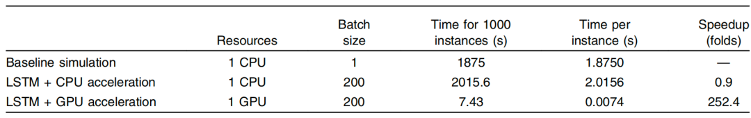
* Running on a single NVIDIA A100 GPU at a batch size of 200, single-sample inference time was reduced to 7.43 milliseconds, a 252x improvement over the SSFM model.

This research bridges the gap between numerical simulation and practical experimental applications, opening up new research avenues for the design of efficient, scalable, and intelligent photonic systems.

Paper address:
https://go.hyper.ai/5bLoA

Constructing a high-fidelity simulation dataset for χ⁽²⁾ nonlinear optics

The dataset used in this study is based on a full-process simulation model of the photocathode-driven laser system of the coherent source at the LCLS-II linear accelerator in the SLAC laboratory. This system includes a 1,035 nm mode-locked infrared laser source, a programmable spectral shaper, a chirped pulse amplifier, and a nonlinear frequency conversion module (as shown in Figure a). To cover a wide range of pulse patterns,The study generated 10,000 pulse shaping configurations by randomly sampling second-order dispersion, third-order dispersion, and spectral amplitude shaping parameters.There were no fewer than 400 configurations using only phase shaping. Each configuration was then subjected to high-precision simulation using SSFM, ultimately yielding three coupled optical field data points on 100 transmission slices in the nonlinear crystal: SHG1, SFG, and SHG2, with a single-field sampling point count of 32,768.

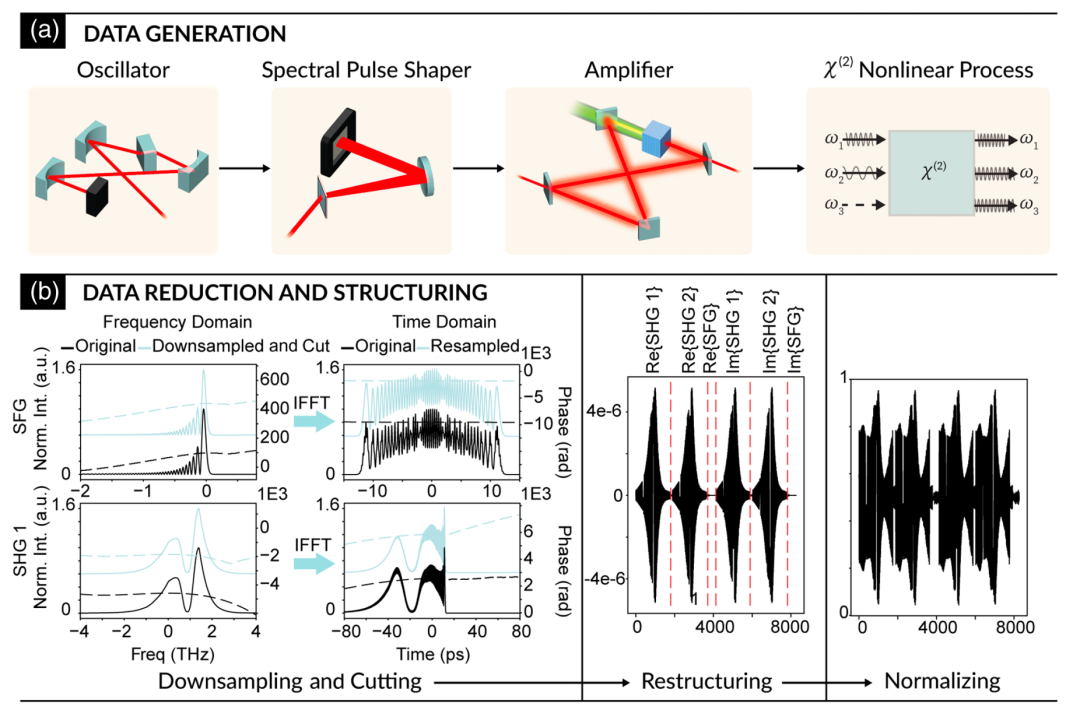
In the data preprocessing stage, the study adopted a three-stage process (as shown in Figure b above): The first stage truncates and downsamples the optical field in the frequency domain, reducing the SFG optical field to 348 complex values and the two SHG optical fields to 1,892 complex values respectively; the second stage concatenates the real and imaginary parts of each optical field to form a real-valued vector with a fixed length of 8,264 elements; the third stage normalizes all elements in the vector to the interval [0,1] based on the extreme values of the global dataset.The final dataset was divided into 890,000 training samples, 10,000 validation samples, and 90,000 test samples.

Building an LSTM-based sequence proxy model architecture

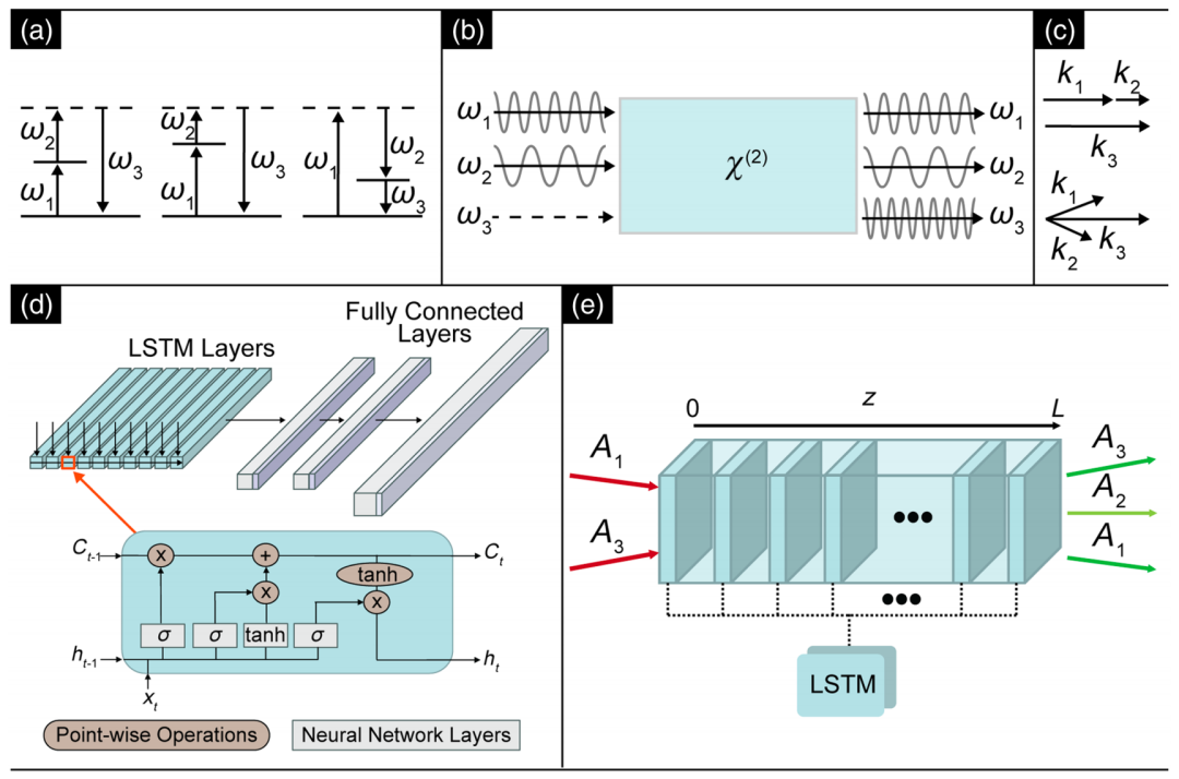
The LSTM model uses a sequence-to-sequence architecture, treating each discrete slice of the nonlinear crystal as a time step.This network contains 2,048 hidden units, followed by three fully connected layers with dimensions of (2048, 4096), (4096, 4096), and (4096, 8264), respectively. The three fully connected layers use ReLU, Tanh, and Sigmoid activations, as shown in the figure below.

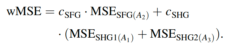
The LSTM model is optimized using the Adam optimizer and the weighted mean squared error (wMSE) loss function, as shown in the figure below:

During training, the LSTM model uses a sequence of 10 spatial slices as input to predict the next slice. For each set of simulated data containing 100 slices, 100 sets of input-output samples are generated by sliding a window across the sequence. The first 9 sets are appended to the beginning of the input sequence to ensure a uniform input length. The final input training tensor shape is (batch size, 10, 8264), and the output tensor shape is (batch size, 8264).

The LSTM model uses an autoregressive approach for inference.First, the initial slice is repeated 10 times as the first input. Then, the LSTM model predicts the next slice and appends it to the end of the input sequence, while discarding the earliest slice in the sequence, always maintaining the input window length at 10. This process is repeated cyclically to complete the derivation for all 100 spatial steps. With the prediction results of the sequence model, the evolution process of the entire field physical quantities inside the nonlinear crystal is fully reconstructed.

Both accuracy and efficiency are improved, with a speedup of 252 times compared to baseline simulation.

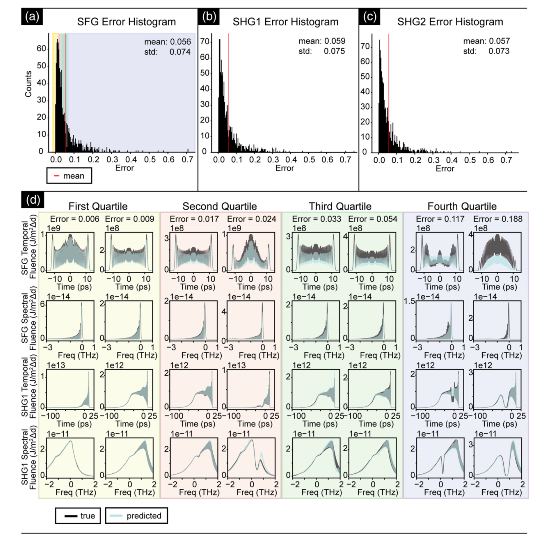
To evaluate the inference performance of the LSTM model,The study employs a comprehensive error index that takes into account both waveform morphology and total energy sensitivity.This comprehensive index comprises three dimensionless components: the cosine similarity of the area-normalized waveform, which is inverted and scaled to ensure zero error when the waveforms are perfectly identical; the normalized mean square error (NMSE) calculated based on the total integral intensity and proportional to the energy, used to penalize energy mismatches; and the Wasserstein distance (Earth Mover's Distance, EMD) between the two sets of intensity distribution curves, which can accurately detect local redistribution of intensity.

Waveform reconstruction accuracy

In terms of experimental setup, the LSTM converged after approximately 180 epochs of training on a single NVIDIA A10G GPU, with a training time of about 160 hours. The final training loss and validation loss reached 2.05 x 10⁻⁵ and 2.03 x 10⁻⁵, respectively. The evaluation method was to calculate the combined error index between the prediction results and the SSFM simulation results.

Regarding the experimental results, to visually present the qualitative effects, the study plotted histograms and statistics of the combined temporal intensity error indices for SFG, SHG1, and SHG2, respectively. Two sets of test datasets were randomly selected from the four quartiles of the SFG error distribution. The predicted and actual intensity curves of SFG and its corresponding SHG1 in the time and frequency domains are presented, as shown in the figure below:

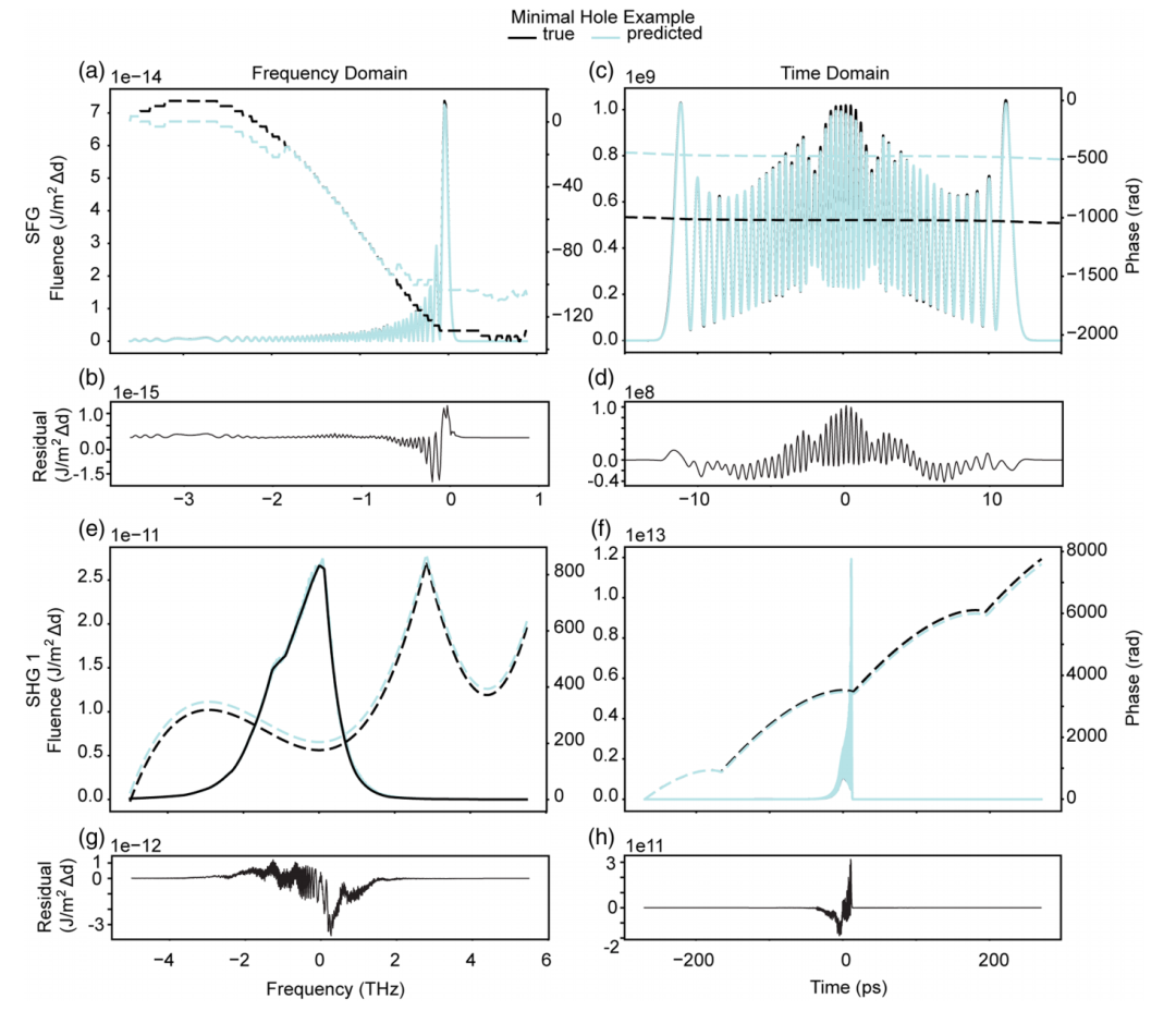
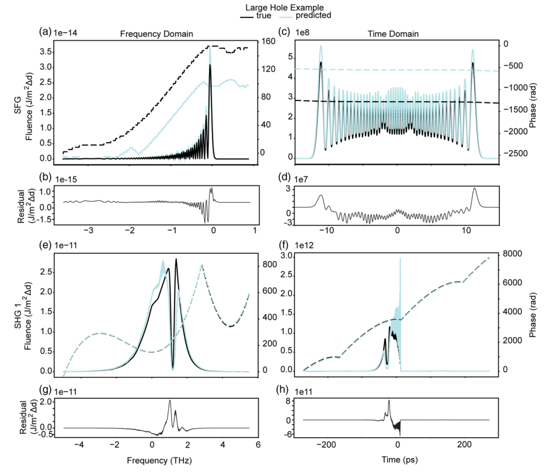
The two sets of images below show two additional examples from the highest quartile of the error distribution, highlighting the performance of the LSTM model under different shaping conditions. The results show that the combined error indices for the two models are 0.012 and 0.003, respectively. Under both conditions,The LSTM models can accurately reconstruct SFG and SHG1 in the frequency or time domain. Only when the spectral modulation amplitude is large will SHG1 show local deviation.These examples demonstrate that the LSTM model can achieve good generalization under various spectral shaping conditions.

Model computational efficiency

The figure below shows the inference time of the LSTM model under different hardware: the baseline simulation is based on the SSFM model, where SSFM solves the main time-consuming terms when solving for nonlinear propagation.Specifically, on a single-core CPU, the complete simulation takes 1.98 seconds, while the SSFM operation takes about 1.875 seconds. The LSTM model takes about the same time as the baseline simulation on a single-core CPU, due to the overhead of batch processing; however, on a single NVIDIA A100 GPU with a batch size of 200, the single-sample inference time is only 7.43 milliseconds, which is 252 times faster than the baseline simulation.

Conclusion

This study is inspired by past experience and incorporates several innovative ideas, such as a three-in-one composite evaluation system that combines inverse cosine similarity, NMSE, and EMD. This system changes the traditional single index, which cannot be adapted to the visual and practical effect evaluation of various pulse morphologies and energy scales, making the experimental results more reliable and credible.

Of course, the most important core advantage of LSTM lies in its complete transformation of the traditional SSFM model, which requires repeated time-frequency domain transformations, resulting in high computational costs. LSTM only needs to learn the mapping relationship directly in the simplified frequency domain, eliminating the need for frequent step-by-step Fourier transforms and enabling real-time derivation. Furthermore, in addition to SFG processes, LSTM models can be applied to various second-order nonlinear optical scenarios, possessing broad application potential and adapting to the needs of current experimental and practical applications.

Finally, the successful validation of the LSTM model further reveals the high-efficiency enabling capability of machine learning models in the field of nonlinear optical simulation, breaking down the barriers between pure numerical simulation and physical experiments, and providing a new technical paradigm for the design of efficient, large-scale, and intelligent optoelectronic systems.