Command Palette
Search for a command to run...
Practical Experience | Elementwise Operator Optimization Practice Based on HyperAI Cloud Computing Platform

The HyperAI computing platform has been officially launched, providing developers with highly stable computing services and accelerating the realization of their ideas through an out-of-the-box environment, cost-effective GPU pricing, and abundant on-site resources.
The following is a sharing of HyperAI users' experiences in optimizing Elementwise operators based on the platform ⬇️
A quick announcement about an event!
The HyperAI beta testing program is still recruiting, with a maximum incentive of $200. Click to learn more about the program:Up to $200 can be obtained! HyperAI beta test recruitment is officially open!
Core objective:Optimize a simple element-wise addition operator (C = A + B) from its basic implementation to approach the native performance of PyTorch (i.e., approach the hardware's memory bandwidth limit).
Key challenges:Elementwise is a typical memory bound operator.
- Computing power is not the bottleneck (GPUs perform addition incredibly fast).
- The bottleneck lies in the supply and demand balance of the "instruction issuing end" and the "video memory transport end".
- The essence of optimization is to move the most data (bytes) with the fewest instructions.
Experimental Environment and Computing Power Preparation
The optimization of the Elementwise operator essentially pushes the physical limits of GPU memory bandwidth. To obtain the most accurate benchmark data, this practical exercise was conducted on HyperAI's (hyper.ai) cloud computing platform. I specifically chose a high-spec instance to squeeze the most out of the operator's performance:
- GPU: NVIDIA RTX 5090 (32GB VRAM)
- RAM: 40 GB
- Environment: PyTorch 2.8 / CUDA 12.8
Bonus Time: If you also want to experience the RTX 5090 and reproduce the code in this article, you can use my exclusive redemption code "EARLY_dnbyl" when registering app.hyper.ai to receive 1 hour of free 5090 computing power (valid for 1 month).
Quickly launch an RTX 5090 instance
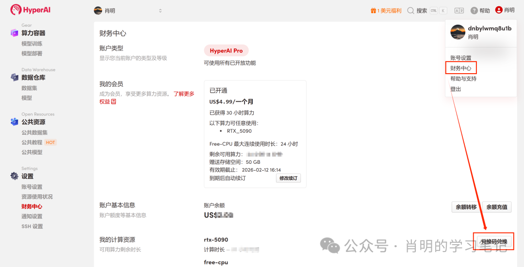
1. Registration and Login: After registering an account at app.hyper.ai, click "Financial Center" in the upper right corner, then click "Redeem Code" and enter "EARLY_dnbyl" to receive free computing power.
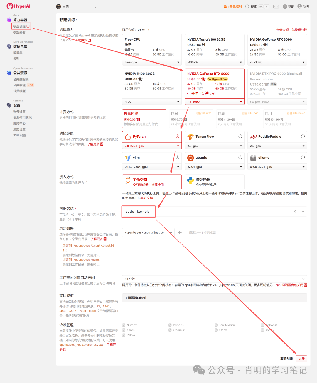
2. Create a container: Click "Model Training" in the left sidebar -> "Select Computing Power: 5090" -> "Select Image: PyTorch 2.8" -> "Access Method: Jupyter" -> "Container Name: Enter anything, such as cuda_kernels" -> "Execute".
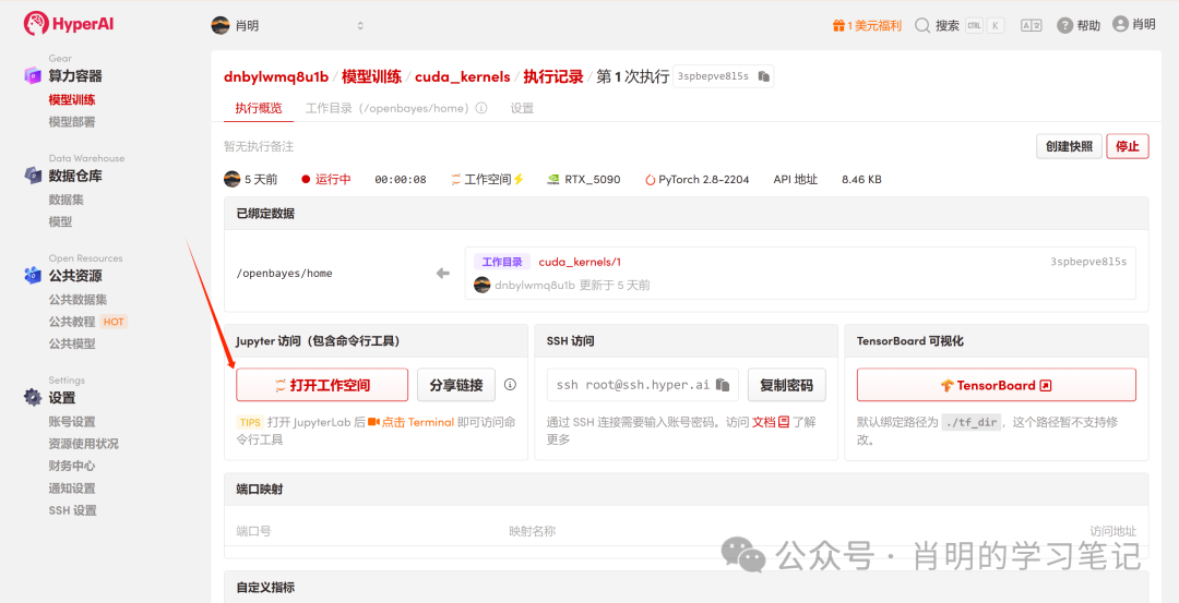
3. Open Jupyter: After the instance starts (its status changes to "Running"), simply click "Open Workspace" to use it immediately.
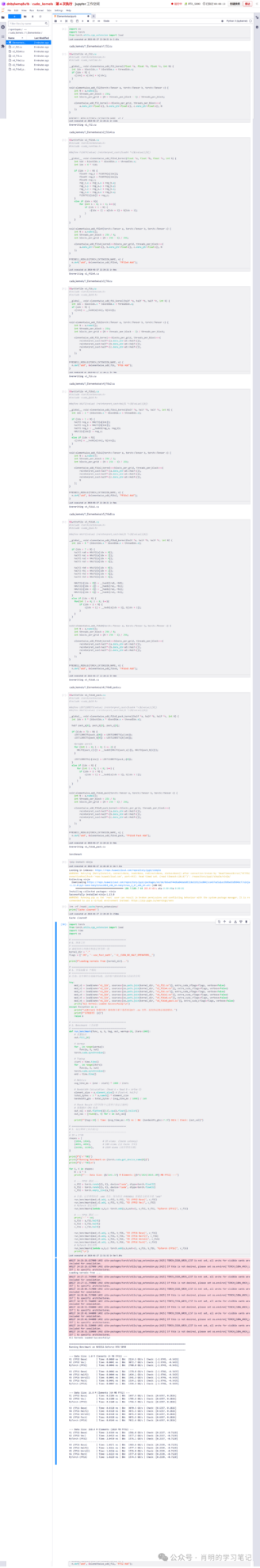
The platform supports connecting using Jupyter or VS Code SSH Remote. I'm using Jupyter, and I ran the following command in the first cell:
import os
import torch
from torch.utils.cpp_extension import load
Phase 1: FP32 Optimization Series
Version 1: FP32 Baseline (Scalar Version)
This is the most intuitive way to write it, but it's only so-so in terms of efficiency from the GPU's perspective.
In-depth analysis of the principles:
- Command layer:The Scheduler issues one LD.E (32-bit Load) instruction.
- Execution layer (Warp)According to the SIMT principle, all 32 threads in the Warp execute this instruction simultaneously.
- Data volume:Each thread moves 4 bytes. Total data volume =32 threads × 4 Bytes = 128 Bytes .
- Memory transactions:The LSU (Load Store Unit) combines these 128 bytes into one video memory transaction.
- Bottleneck analysis:Although memory merging is utilized, instruction efficiency is low. To move 128 bytes of data, the SM (Streaming Multiprocessor) must consume one instruction issue cycle. For massive amounts of data, the instruction issue unit becomes overwhelmed and becomes a bottleneck.
Code (v1_f32.cu):
%%writefile v1_f32.cu
  #include <torch/extension.h>
  #include <cuda_runtime.h>

  __global__ void elementwise_add_f32_kernel(float *a, float *b, float *c, int N) {
  int idx = blockIdx.x * blockDim.x + threadIdx.x;
  if (idx < N) {
  c[idx] = a[idx] + b[idx];
  }
}

void elementwise_add_f32(torch::Tensor a, torch::Tensor b, torch::Tensor c) {
  int N = a.numel();
  int threads_per_block = 256;
  int blocks_per_grid = (N + threads_per_block - 1) / threads_per_block;

  elementwise_add_f32_kernel<<<blocks_per_grid, threads_per_block>>>(
  a.data_ptr<float>(), b.data_ptr<float>(), c.data_ptr<float>(), N
  );
}

  PYBIND11_MODULE(TORCH_EXTENSION_NAME, m) {
  m.def("add", &elementwise_add_f32, "FP32 Add");
}
Version 2: FP32x4 Vectorized
Optimization method: Use the float4 type to force the generation of 128-bit load instructions.
In-depth analysis of the principles (core optimization points):
- Command layer:The Scheduler issues one LD.E.128 (128-bit Load) instruction.
- Execution layer (Warp):The warp has 32 threads running simultaneously, but this time each thread moves 16 bytes (float4).
- Data volume:Total data volume = 32 threads x 16 Bytes = 512 Bytes.
- Memory transactions:When the LSU sees a continuous request of 512 bytes, it will initiate four consecutive 128-byte memory transactions.
- Efficiency comparison:Baseline: 1 instruction = 128 bytes. Vectorized: 1 instruction = 512 bytes.
- in conclusion:Instruction efficiency is improved by 4 times. SM only requires 1/4 of the original number of instructions to fully utilize the same memory bandwidth. This completely frees up the instruction dispatch unit, truly shifting the bottleneck to memory bandwidth.
Code (v2_f32x4.cu):
%%writefile v2_f32x4.cu
#include <torch/extension.h>
#include <cuda_runtime.h>

#define FLOAT4(value) (reinterpret_cast<float4 *>(&(value))[0])

__global__ void elementwise_add_f32x4_kernel(float *a, float *b, float *c, int N) {
  int tid = blockIdx.x * blockDim.x + threadIdx.x;
  int idx = 4 * tid;

  if (idx + 3 < N) {
    float4 reg_a = FLOAT4(a[idx]);
    float4 reg_b = FLOAT4(b[idx]);
    float4 reg_c;
    reg_c.x = reg_a.x + reg_b.x;
    reg_c.y = reg_a.y + reg_b.y;
    reg_c.z = reg_a.z + reg_b.z;
    reg_c.w = reg_a.w + reg_b.w;
    FLOAT4(c[idx]) = reg_c;
  }
  else if (idx < N){
    for (int i = 0; i < 4; i++){
      if (idx + i < N) {
        c[idx + i] = a[idx + i] + b[idx + i];
      }
    }
  }
}

void elementwise_add_f32x4(torch::Tensor a, torch::Tensor b, torch::Tensor c) {
  int N = a.numel();
  int threads_per_block = 256 / 4;
  int blocks_per_grid = (N + 256 - 1) / 256;

  elementwise_add_f32x4_kernel<<<blocks_per_grid, threads_per_block>>>(
    a.data_ptr<float>(), b.data_ptr<float>(), c.data_ptr<float>(), N
  );
}

PYBIND11_MODULE(TORCH_EXTENSION_NAME, m) {
  m.def("add", &elementwise_add_f32x4, "FP32x4 Add");
Phase Two: FP16 Optimization Series
3. Version 3: FP16 Baseline (Half-precision scalar)
Use half (FP16) to save video memory.
In-depth analysis of the underlying principles (Why is it so slow?):
- Memory access mode:In the code, idx is consecutive, so access by 32 threads is completely merged.
- Data volume:32 threads × 2 bytes = 64 bytes (total requests for one warp).
- Hardware behavior:The memory controller (LSU) generates two 32-byte memory sector transactions. Note: No bandwidth is wasted here; all transmitted data is valid.
The real bottleneck:
1. Instruction Bound:
This is the core reason. In order to fill the video memory bandwidth, we need to continuously move data.In this version, one instruction can only move 64 bytes.Compared to the float4 version (which moves 512 bytes per instruction), this version's instruction efficiency is only 1/8.
as a result ofEven when the SM's instruction dispatcher is running at full speed, the amount of data carried by the issued instructions cannot fully utilize the enormous video memory bandwidth. It's like the foreman shouting himself hoarse (issuing instructions), but the workers still can't move enough bricks (data).
2. The granularity of memory transactions is too small:
* Physical layer:The smallest unit of video memory transfer is a 32-byte sector; cache layers are typically managed in units of 128-byte cache lines.
* status quo:Although the 64B of data requested by the Warp filled two sectors, it only used half of the 128B cache line.
* as a result of:This "retail-style" small-packet data transfer is extremely inefficient at this throughput compared to the "wholesale" transfer of four complete cache lines (512B) at once, as is done with float4, and it cannot mask the high latency of the video memory. To fill the video memory bandwidth, we need to continuously transfer data.
Code (v3_f16.cu):
%%writefile v3_f16.cu
#include <torch/extension.h>
#include <cuda_fp16.h>

__global__ void elementwise_add_f16_kernel(half *a, half *b, half *c, int N) {
int idx = blockIdx.x * blockDim.x + threadIdx.x;
if (idx < N) {
        c[idx] = __hadd(a[idx], b[idx]);
    }
}

void elementwise_add_f16(torch::Tensor a, torch::Tensor b, torch::Tensor c) {      int N = a.numel();
      int threads_per_block = 256;
      int blocks_per_grid = (N + threads_per_block - 1) / threads_per_block;

elementwise_add_f16_kernel<<<blocks_per_grid, threads_per_block>>>(             reinterpret_cast<half*>(a.data_ptr<at::Half>()),
            reinterpret_cast<half*>(b.data_ptr<at::Half>()),
            reinterpret_cast<half*>(c.data_ptr<at::Half>()),
 N
      );
}
PYBIND11_MODULE(TORCH_EXTENSION_NAME, m) {
    m.def("add", &elementwise_add_f16, "FP16 Add");
}
4.Version 4: FP16 Vectorized (Half2)
Introduce half2.
In-depth analysis of the principles:
- data:half2 (4 bytes).
- Command layer:Issue a 32-bit Load command.
- Computing layer:Using __hadd2 (SIMD), a single instruction can perform two additions simultaneously.
- status quo:Memory access efficiency is equivalent to FP32 Baseline(1 instruction = 128 bytes). Although it is faster than V3, it still does not reach the peak of 512 bytes/instruction of float4.
Code (v4_f16x2.cu):
%%writefile v3_f16.cu
#include <torch/extension.h>
#include <cuda_fp16.h>

__global__ void elementwise_add_f16_kernel(half *a, half *b, half *c, int N) {
  int idx = blockIdx.x * blockDim.x + threadIdx.x;
  if (idx < N) {
    c[idx] = __hadd(a[idx], b[idx]);
  }
}

void elementwise_add_f16(torch::Tensor a, torch::Tensor b, torch::Tensor c) {
  int N = a.numel();
  int threads_per_block = 256;
  int blocks_per_grid = (N + threads_per_block - 1) / threads_per_block;

  elementwise_add_f16_kernel<<<blocks_per_grid, threads_per_block>>>(
    reinterpret_cast<half*>(a.data_ptr<at::Half>()),
    reinterpret_cast<half*>(b.data_ptr<at::Half>()),
    reinterpret_cast<half*>(c.data_ptr<at::Half>()),
    N
  );
}

PYBIND11_MODULE(TORCH_EXTENSION_NAME, m) {
  m.def("add", &elementwise_add_f16, "FP16 Add");
}
See the appendix for a sample of running hyper Jupyter.
5. Version 5: FP16x8 Unroll (Manual Loop Unroll)
To further explore performance, we tried having one thread handle eight halfs (i.e., four half2s).
In-depth analysis of the underlying principles (where are the improvements compared to V4?):
- practice:Manually write four consecutive lines of half2 read operations in the code.
- Effect:The Scheduler will issue four 32-bit Load commands in succession.
- income:ILP (Instruction-Level Parallelism) and Latency Masking. Issues with V4 (FP16x2):Issue one instruction -> wait for data to return (Stall) -> perform calculation. During the waiting period, the GPU does nothing. Improvements in V5:It issues four instructions in quick succession. While the GPU is still waiting for the first data to return from memory, it has already issued the second, third, and fourth instructions. This fully utilizes the gaps in the instruction pipeline, masking the expensive memory latency.
- Limitations:The instruction density remains very high.Although ILP was utilized, it essentially still initiated four 32-bit "cart transports". To move 128 bits of data, SM still consumed four instruction issue cycles. The instruction issuer remained very busy, failing to achieve the effect of "moving a mountain with one instruction".
Code (v5_f16x8.cu):
%%writefile v5_f16x8.cu
#include <torch/extension.h>
#include <cuda_fp16.h>

#define HALF2(value) (reinterpret_cast<half2 *>(&(value))[0])

__global__ void elementwise_add_f16x8_kernel(half *a, half *b, half *c, int N) {
  int idx = 8 * (blockIdx.x * blockDim.x + threadIdx.x);

  if (idx + 7 < N) {
    half2 ra0 = HALF2(a[idx + 0]);
    half2 ra1 = HALF2(a[idx + 2]);
    half2 ra2 = HALF2(a[idx + 4]);
    half2 ra3 = HALF2(a[idx + 6]);

    half2 rb0 = HALF2(b[idx + 0]);
    half2 rb1 = HALF2(b[idx + 2]);
    half2 rb2 = HALF2(b[idx + 4]);
    half2 rb3 = HALF2(b[idx + 6]);

    HALF2(c[idx + 0]) = __hadd2(ra0, rb0);
    HALF2(c[idx + 2]) = __hadd2(ra1, rb1);
    HALF2(c[idx + 4]) = __hadd2(ra2, rb2);
    HALF2(c[idx + 6]) = __hadd2(ra3, rb3);
  }
  else if (idx < N) {
    for(int i = 0; i < 8; i++){
      if (idx + i < N) {
        c[idx + i] = __hadd(a[idx + i], b[idx + i]);
      }
    }
  }
}

void elementwise_add_f16x8(torch::Tensor a, torch::Tensor b, torch::Tensor c) {
  int N = a.numel();
  int threads_per_block = 256 / 8;
  int blocks_per_grid = (N + 256 - 1) / 256;

  elementwise_add_f16x8_kernel<<<blocks_per_grid, threads_per_block>>>(
    reinterpret_cast<half*>(a.data_ptr<at::Half>()),
    reinterpret_cast<half*>(b.data_ptr<at::Half>()),
    reinterpret_cast<half*>(c.data_ptr<at::Half>()),
    N
  );
}

PYBIND11_MODULE(TORCH_EXTENSION_NAME, m) {
  m.def("add", &elementwise_add_f16x8, "FP16x8 Add");
}
See the appendix for a sample of running hyper Jupyter.
Version 6: FP16x8 Pack (Ultimate Optimization)
This is the ceiling for Elementwise operator optimization. We combine the "high bandwidth transport" of V2 with the "instruction-level parallelism" of V5, and introduce register caching technology.
In-depth analysis of core magic:
1. Address spoofing:
* question:Our data is of type half, and the GPU does not have a native load_8_halfs instruction.
* Countermeasures: The float4 type occupies exactly 128 bits (16 bytes), and 8 halfs also occupy 128 bits.
* operate:We forcibly cast the address of the half array (reinterpret_cast) to float4*.
* Effect:When the compiler sees `float4*`, it will generate one line. LD.E.128 Instructions. The video memory controller doesn't care what you're moving; it only moves 128-bit binary streams at a time.
2. Register Array:
half pack_a[8]: Although this array is defined in the kernel, because it is of fixed size and very small, the compiler will directly map it to the GPU's register file instead of the slow local memory. This is equivalent to opening up a high-speed cache "on hand".
3. Memory Reinterpretation:
Macro definition LDST128BITS:This is the soul of the code. It casts the address of any variable to a float4* and retrieves its value.
LDST128BITS(pack_a[0])=LDST128BITS(a[idx]);
* Right side:Go to Global Memory a[idx] and retrieve 128 bits of data.
* leftWrite this 128-bit data directly into the pack_a array (starting from the 0th element, filling all 8 elements instantly).
* result:One instruction instantly completes the transfer of 8 data items.
Code (v6_f16x8_pack.cu):
%%writefile v6_f16x8_pack.cu
#include <torch/extension.h>
#include <cuda_fp16.h>

#define LDST128BITS(value) (reinterpret_cast<float4 *>(&(value))[0])
#define HALF2(value) (reinterpret_cast<half2 *>(&(value))[0])

__global__ void elementwise_add_f16x8_pack_kernel(half *a, half *b, half *c, int N) {
  int idx = 8 * (blockIdx.x * blockDim.x + threadIdx.x);

  half pack_a[8], pack_b[8], pack_c[8];

  if ((idx + 7) < N) {
    LDST128BITS(pack_a[0]) = LDST128BITS(a[idx]);
    LDST128BITS(pack_b[0]) = LDST128BITS(b[idx]);

    #pragma unroll
    for (int i = 0; i < 8; i += 2) {
      HALF2(pack_c[i]) = __hadd2(HALF2(pack_a[i]), HALF2(pack_b[i]));
    }

    LDST128BITS(c[idx]) = LDST128BITS(pack_c[0]);
  }
  else if (idx < N) {
    for (int i = 0; i < 8; i++) {
      if (idx + i < N) {
        c[idx + i] = __hadd(a[idx + i], b[idx + i]);
      }
    }
   }
 }

 void elementwise_add_f16x8_pack(torch::Tensor a, torch::Tensor b, torch::Tensor c) {
   int N = a.numel();
   int threads_per_block = 256 / 8;
   int blocks_per_grid = (N + 256 - 1) / 256;

   elementwise_add_f16x8_pack_kernel<<<blocks_per_grid, threads_per_block>>>(
     reinterpret_cast<half*>(a.data_ptr<at::Half>()),
     reinterpret_cast<half*>(b.data_ptr<at::Half>()),
     reinterpret_cast<half*>(c.data_ptr<at::Half>()),
     N
   );
 }

 PYBIND11_MODULE(TORCH_EXTENSION_NAME, m) {
   m.def("add", &elementwise_add_f16x8_pack, "FP16x8 Pack Add");
 }
Phase 3: Combining Benchmarks and Visual Analysis
To comprehensively evaluate the optimization effect, we designed a full-scenario test plan covering latency-sensitive (small data) to bandwidth-sensitive (big data) scenarios.
1. Test strategy design
We selected three representative datasets, each corresponding to different bottlenecks at the GPU memory level:
- Cache Latency (1M elements):The data size is extremely small (4MB), and the L2 cache is fully hit.The core of the test is Kernel launch overhead and command issuance efficiency.
- L2 Throughput (16M elements):The data size is moderate (64MB), close to the L2 cache capacity limit.The core of the test is the read and write throughput of the L2 cache.
- VRAM Bandwidth (256M elements):The data volume is enormous (1GB), far exceeding the L2 cache. The data must be moved from the video memory (VRAM).This is the real battlefield for large-scale operators; the core test lies in whether the physical memory bandwidth is fully utilized.
2. Benchmark script (Python)
The script directly loads the .cu file defined above and automatically calculates the bandwidth (GB/s) and latency (ms).
import torch
from torch.utils.cpp_extension import load
import time
import os

# ==========================================
# 0. 准备工作
# ==========================================
# 确保你的文件路径和笔记里写的一致
kernel_dir = "."
flags = ["-O3", "--use_fast_math", "-U__CUDA_NO_HALF_OPERATORS__"]

print(f"Loading kernels from {kernel_dir}...")

# ==========================================
# 1. 分别加载 6 个模块
# ==========================================
# 我们分别编译加载,确保每个模块有独立的命名空间,避免符号冲突
try:
  mod_v1 = load(name="v1_lib", sources=[os.path.join(kernel_dir, "v1_f32.cu")], extra_cuda_cflags=flags, verbose=False)
  mod_v2 = load(name="v2_lib", sources=[os.path.join(kernel_dir, "v2_f32x4.cu")], extra_cuda_cflags=flags, verbose=False)
  mod_v3 = load(name="v3_lib", sources=[os.path.join(kernel_dir, "v3_f16.cu")], extra_cuda_cflags=flags, verbose=False)
  mod_v4 = load(name="v4_lib", sources=[os.path.join(kernel_dir, "v4_f16x2.cu")], extra_cuda_cflags=flags, verbose=False)
  mod_v5 = load(name="v5_lib", sources=[os.path.join(kernel_dir, "v5_f16x8.cu")], extra_cuda_cflags=flags, verbose=False)
  mod_v6 = load(name="v6_lib", sources=[os.path.join(kernel_dir, "v6_f16x8_pack.cu")], extra_cuda_cflags=flags, verbose=False)
  print("All Kernels Loaded Successfully!\n")
except Exception as e:
  print("\n[Error] 加载失败!请检查目录下是否有这 6 个 .cu 文件,且代码已修正语法错误。")
  print(f"详细报错: {e}")
  raise e

# ==========================================
# 2. Benchmark 工具函数
# ==========================================
def run_benchmark(func, a, b, tag, out, warmup=10, iters=1000):
  # 重置输出
  out.fill_(0)

  # Warmup (预热,让 GPU 进入高性能状态)
  for _ in range(warmup):
    func(a, b, out)
  torch.cuda.synchronize()

  # Timing (计时)
  start = time.time()
  for _ in range(iters):
    func(a, b, out)
  torch.cuda.synchronize()
  end = time.time()

  # Metrics (指标计算)
  avg_time_ms = (end - start) * 1000 / iters

  # Bandwidth Calculation: (Read A + Read B + Write C)
  element_size = a.element_size() # float=4, half=2
  total_bytes = 3 * a.numel() * element_size
  bandwidth_gbs = total_bytes / (avg_time_ms / 1000) / 1e9

  # Check Result (打印前 2 个元素用于验证正确性)
  # 取数据回 CPU 检查
  out_val = out.flatten()[:2].cpu().float().tolist()
  out_val = [round(v, 4) for v in out_val]

  print(f"{tag:<20} | Time: {avg_time_ms:.4f} ms | BW: {bandwidth_gbs:>7.1f} GB/s | Check: {out_val}")

  # ==========================================
  # 3. 运行测试 (从小到大)
  # ==========================================
  # 1M = 2^20
  shapes = [
    (1024, 1024),         # 1M elems  (Cache Latency)
    (4096, 4096),         # 16M elems (L2 Cache 吞吐)
    (16384, 16384),       # 256M elems (显存带宽压测)
  ]

  print(f"{'='*90}")
  print(f"Running Benchmark on {torch.cuda.get_device_name(0)}")
  print(f"{'='*90}\n")

  for S, K in shapes:
    N = S * K
    print(f"--- Data Size: {N/1e6:.1f} M Elements ({N*4/1024/1024:.0f} MB FP32) ---")

    # --- FP32 测试 ---
    a_f32 = torch.randn((S, K), device="cuda", dtype=torch.float32)
    b_f32 = torch.randn((S, K), device="cuda", dtype=torch.float32)
    c_f32 = torch.empty_like(a_f32)

    # 注意:这里调用的是 .add 方法,因为你在 PYBIND11 里面定义的名字是 "add"
    run_benchmark(mod_v1.add, a_f32, b_f32, "V1 (FP32 Base)", c_f32)
    run_benchmark(mod_v2.add, a_f32, b_f32, "V2 (FP32 Vec)", c_f32)
    # PyTorch 原生对照
    run_benchmark(lambda a,b,c: torch.add(a,b,out=c), a_f32, b_f32, "PyTorch (FP32)", c_f32)

    # --- FP16 测试 ---
    print("-" * 60)
    a_f16 = a_f32.half()
    b_f16 = b_f32.half()
    c_f16 = c_f32.half()

    run_benchmark(mod_v3.add, a_f16, b_f16, "V3 (FP16 Base)", c_f16)
    run_benchmark(mod_v4.add, a_f16, b_f16, "V4 (FP16 Half2)", c_f16)
    run_benchmark(mod_v5.add, a_f16, b_f16, "V5 (FP16 Unroll)", c_f16)
    run_benchmark(mod_v6.add, a_f16, b_f16, "V6 (FP16 Pack)", c_f16)
    # PyTorch 原生对照
    run_benchmark(lambda a,b,c: torch.add(a,b,out=c), a_f16, b_f16, "PyTorch (FP16)", c_f16)
    print("\n")
3. Real-world data: RTX 5090 performance
The following are the actual data obtained by running the above code on an NVIDIA GeForce RTX 5090:
==========================================================================================
Running Benchmark on NVIDIA GeForce RTX 5090
==========================================================================================---

Data Size: 1.0 M Elements (4 MB FP32) ---
V1 (FP32 Base)       | Time: 0.0041 ms | BW:  3063.1 GB/s | Check: [0.8656, 1.9516]
V2 (FP32 Vec)        | Time: 0.0041 ms | BW:  3066.1 GB/s | Check: [0.8656, 1.9516]
PyTorch (FP32)       | Time: 0.0044 ms | BW:  2868.9 GB/s | Check: [0.8656, 1.9516]
------------------------------------------------------------
V3 (FP16 Base)       | Time: 0.0041 ms | BW:  1531.9 GB/s | Check: [0.8657, 1.9512]
V4 (FP16 Half2)      | Time: 0.0041 ms | BW:  1531.9 GB/s | Check: [0.8657, 1.9512]
V5 (FP16 Unroll)     | Time: 0.0041 ms | BW:  1533.5 GB/s | Check: [0.8657, 1.9512]
V6 (FP16 Pack)       | Time: 0.0041 ms | BW:  1533.6 GB/s | Check: [0.8657, 1.9512]
PyTorch (FP16)       | Time: 0.0044 ms | BW:  1431.6 GB/s | Check: [0.8657, 1.9512]


--- Data Size: 16.8 M Elements (64 MB FP32) ---
V1 (FP32 Base)       | Time: 0.1183 ms | BW:  1702.2 GB/s | Check: [-3.2359, -0.1663]
V2 (FP32 Vec)        | Time: 0.1186 ms | BW:  1698.1 GB/s | Check: [-3.2359, -0.1663]
PyTorch (FP32)       | Time: 0.1176 ms | BW:  1711.8 GB/s | Check: [-3.2359, -0.1663]
------------------------------------------------------------
V3 (FP16 Base)       | Time: 0.0348 ms | BW:  2891.3 GB/s | Check: [-3.2363, -0.1664]
V4 (FP16 Half2)      | Time: 0.0348 ms | BW:  2891.3 GB/s | Check: [-3.2363, -0.1664]
V5 (FP16 Unroll)     | Time: 0.0348 ms | BW:  2892.8 GB/s | Check: [-3.2363, -0.1664]
V6 (FP16 Pack)       | Time: 0.0348 ms | BW:  2892.6 GB/s | Check: [-3.2363, -0.1664]
PyTorch (FP16)       | Time: 0.0148 ms | BW:  6815.7 GB/s | Check: [-3.2363, -0.1664]


--- Data Size: 268.4 M Elements (1024 MB FP32) ---
V1 (FP32 Base)       | Time: 2.0432 ms | BW:  1576.5 GB/s | Check: [0.4839, -2.6795]
V2 (FP32 Vec)        | Time: 2.0450 ms | BW:  1575.2 GB/s | Check: [0.4839, -2.6795]
PyTorch (FP32)       | Time: 2.0462 ms | BW:  1574.3 GB/s | Check: [0.4839, -2.6795]
------------------------------------------------------------
V3 (FP16 Base)       | Time: 1.0173 ms | BW:  1583.2 GB/s | Check: [0.4839, -2.6797]
V4 (FP16 Half2)      | Time: 1.0249 ms | BW:  1571.5 GB/s | Check: [0.4839, -2.6797]
V5 (FP16 Unroll)     | Time: 1.0235 ms | BW:  1573.6 GB/s | Check: [0.4839, -2.6797]
V6 (FP16 Pack)       | Time: 1.0236 ms | BW:  1573.4 GB/s | Check: [0.4839, -2.6797]
PyTorch (FP16)       | Time: 1.0251 ms | BW:  1571.2 GB/s | Check: [0.4839, -2.6797]
4. Data Interpretation
This data clearly demonstrates the physical characteristics of the RTX 5090 under different loads:
Phase 1: Very small scale (1M Elements / 4MB)
- Phenomenon:All versions had a remarkably consistent execution time of 0.0041 ms.
- the truth:This is a latency-bound situation. Regardless of the data size, the fixed launch overhead for the GPU to start a kernel is approximately 4 microseconds. Because of this time-limited limitation, the data volume for FP16 is only half that of FP32, so the calculated bandwidth is naturally only half. What is being measured here is not the transmission speed, but the "launch speed".
Phase Two: Medium Size (16M Elements / 64MB vs 32MB)
This is the area that best demonstrates the function of L2 cache:
- FP32 (64MB):The total data volume A+B+C ≈ 192MB. This exceeds the L2 cache capacity of the RTX 5090 (approximately 128MB). Data overflow forced the system to read and write to VRAM, causing the bandwidth to drop to 1700 GB/s (close to the physical bandwidth of the video memory).
- FP16 (32MB):Total data volume.It fits perfectly into the L2 cache! The data circulates within the cache, causing bandwidth to surge to 2890 GB/s.
- The Dark Magic of PyTorch:Note that PyTorch achieved 6815 GB/s in FP16. This demonstrates that in a pure cache scenario, the instruction pipeline optimization of the JIT compiler is still superior to a simple hand-written kernel.
Phase 3: Large-scale (268M Elements / 1024MB)
This is a real-world scenario for training/inference with a large model (Memory Bound):
- All beings are equal:Whether it's FP32 or FP16, whether it's Baseline or Optimized, the bandwidth is all locked at 1570-1580 GB/s.
- Physical wall:We've successfully reached the physical limit of the RTX 5090's GDDR7 memory bandwidth. The bandwidth is limited; nothing can be increased.
- The value of optimization:Although the bandwidth remained the same.However, it was found that the FP16 time (1.02ms) was only half that of the FP32 (2.04ms).By halving the data volume while maximizing bandwidth, there is a 2x end-to-end acceleration. V6 vs V3While V3 appears to run at full capacity, this is due to automatic optimization by the NVCC compiler and GPU hardware latency masking. However, in more complex operators (such as FlashAttention), the V6 implementation guarantees performance.
Core FAQ: Hardcore Derivation of Parameter Design
In all kernels of this experiment, we unanimously set the parameter: threads_per_block = 256. This number was not randomly selected, but rather a mathematically optimal solution between hardware limitations and scheduling efficiency.
Q: Why is threads_per_block always set to 128 or 256?
A: This is a "golden range" obtained through four layers of screening.
We view the selection process of block_size as a funnel, filtering layer by layer:
1. Warp Alignment -> Must be a multiple of 32
The smallest unit of execution in a GPU is a warp (thread bundle), which consists of 32 consecutive threads (SIMT architecture, single instruction multithreading).
- Hard limitations:If you request 31 threads, the hardware will still schedule one complete warp. Although the remaining thread position is idle, it still occupies the same hardware resources.
- in conclusion: The block_size should ideally be a multiple of 32 to avoid wasting computing power.
2. Occupancy Floor -> Must be >= 96
Occupancy = Number of concurrent threads currently executing on SM / Maximum number of threads supported by SM.
- background:To mask memory latency, we need a sufficient number of active warps. If the block size is too small, the SM's "Max Blocks" limit will be reached before the "Max Threads" limit.
- Estimation:Mainstream architectures (such as Turing/Ampere/Ada) typically require: block_size > (maximum number of threads in the SM / maximum number of blocks in the SM). Common ratios are 64 or 96.
- in conclusion:To theoretically achieve 100% Occupancy, the block size should not be less than 96.
3. Scheduling Atomicity -> Locking 128, 256, 512
A block is the smallest atomic unit scheduled to a SM. The SM must be able to completely consume an integer number of blocks.
- Divisibility:To avoid wasting the capacity of the SM, the block_size should ideally be divisible by the maximum thread capacity of the SM.
- filter:The maximum capacity of mainstream architecture SMs is typically 1024, 1536, 2048, etc. Their common divisor is usually 512. Combining the previous two steps (>=96 and a multiple of 32), our candidate list is narrowed down to: 128, 192, 256, 384, 512.
4. Register Pressure -> Exclude 512+
This is the final "ceiling".
- Hard limitations:The total number of registers available for each block is limited (the total number of registers in the SM is typically 64K 32-bit).
- risk:If the block_size is large (e.g., 512), and the kernel is slightly more complex (each thread uses several registers), then the situation will occur where 512 * Regs/Thread > Max_Regs_Per_Block.
- as a result of:Startup failed: Direct error message. Register Spill: Registers overflow into slow local memory, causing a performance cascade.
- in conclusion:For safety reasons, we generally avoid using 512 or 1024. 128 and 256 are the safest "dessert areas".
Summarize
After four rounds of elimination, only two contestants remained:
- 128It has the strongest versatility.Even with a complex kernel (using many registers), it can still guarantee successful startup and good occupancy.
- 256:elementwise operator preferredFor logically simple operators like element-wise, register pressure is minimal. 256 provides better memory merging potential than 128 and reduces block scheduling overhead.
This also explains why, in the naive implementation, once we determine threads_per_block = 256, grid_size is also determined (as long as the total amount covers N).
Appendix: Jupyter running examples