One-sentence Summary

Researchers at New York University and the Flatiron Institute propose Polar Express, a GPU-friendly polar decomposition method that solves a minimax optimization problem at each iteration to achieve provably optimal worst-case convergence in both early and asymptotic regimes, and demonstrate consistent validation loss improvements over recent alternatives when integrated into the Muon optimizer for GPT-2 training.

Key Contributions

• Polar Express introduces a polar decomposition method that adapts polynomial updates at each iteration by solving a minimax problem and uses only matrix-matrix multiplications, making it efficient for GPU-based Muon optimizers.
• The polynomial sequence is proved to give a worst-case optimal approximation to the sign function, with super-exponential convergence and rapid progress within just five to ten iterations.
• An implementation compatible with bfloat16 is evaluated on synthetic matrices, GPT-2 gradient matrices, and Muon-trained GPT-2 models on one to ten billion FineWeb tokens, improving validation loss across learning rates and being adopted in the NanoGPT speedrun.

Introduction

Advanced linear algebra is increasingly central to deep learning, especially in optimizers like Muon, which replaces the usual momentum direction with the polar factor of a gradient-based matrix. This polar factor is equivalent to a matrix sign function for square matrices and gives a steepest-descent direction under the spectral norm. For large language model training, the computation must be fast, GPU-friendly, memory efficient, and mainly useful at low or moderate accuracy.

Prior methods face practical limitations. A direct SVD is too expensive on GPUs, and many classical polar-decomposition methods require matrix inverses, QR factorizations, or other operations that do not parallelize well. Newton-Schulz is attractive because it uses only matrix-matrix products, but it converges slowly at first. Recent heuristic polynomial iterations reach low-accuracy estimates quickly, but they do not converge to the true polar factor.

The authors introduce Polar Express, a new GPU-friendly iterative method for approximating the matrix polar factor. It adapts the polynomial update rule at each iteration, balancing fast early progress and later accuracy. The method uses polynomials designed to optimize the worst-case approximation of the sign function, converges super-exponentially, and can produce useful approximations within a small number of iterations. Applied inside Muon, Polar Express improves GPT-2 training validation loss across learning rates and has been adopted in optimized NanoGPT training workflows.

Method

The authors design the method to compute $\operatorname{polar}(\boldsymbol M)$polar(M) through operations that are efficient on GPUs: linear combinations of matrices and matrix-matrix products. Since matrix products are more expensive than linear combinations, the algorithm is structured to use as few matrix products as possible. For a matrix with singular value decomposition $\boldsymbol M=\boldsymbol U\boldsymbol \Sigma\boldsymbol V^{\top}$M=UΣV⊤, odd powers can be written as

Therefore, for an odd polynomial

the matrix polynomial can be evaluated as

The central design choice is to approximate $\operatorname{polar}(\boldsymbol M)$polar(M) using a composition of lower-degree odd polynomials. The full approximation has the form

and the matrix iterate is generated recursively by

The final matrix $\boldsymbol X_T$XT​ is the approximation to $\operatorname{polar}(\boldsymbol M)$polar(M). If each component polynomial has odd degree $d$d, this composition requires only $O(Td)$O(Td) matrix products. A standard Newton-Schulz iteration is a special case of this framework, but the authors choose the polynomials to minimize the worst-case approximation error.

Given known or estimated lower and upper bounds $\ell$ℓ and $u$u on the singular values of $\boldsymbol M$M, the goal is to find the composition that minimizes the spectral norm error in the worst case. Because

and the spectral norm is unitarily invariant, this reduces to a scalar uniform approximation problem: find a composed odd polynomial $p$p such that $p(x)$p(x) stays as close as possible to $1$1 for all $x\in[\ell,u]$x∈[ℓ,u]. Formally,

The method solves this problem greedily across iterations. For the current interval $[\ell_t,u_t]$[ℓt​,ut​], one odd-degree-$d$d polynomial is chosen to minimize

This polynomial maps the current interval to a new interval

which then becomes the target interval for the next polynomial. The bounds can be updated using

The resulting composition is optimal among all compositions of $T$T odd polynomials of degree $d$d. The final approximation satisfies

When the singular values are normalized so that $\sigma(\boldsymbol M)\subset[\ell,1]$σ(M)⊂[ℓ,1] and $d=2q+1$d=2q+1, the error bound takes the stronger form

which shows rapidly improving convergence as $T$T grows.

As shown in the figure below:

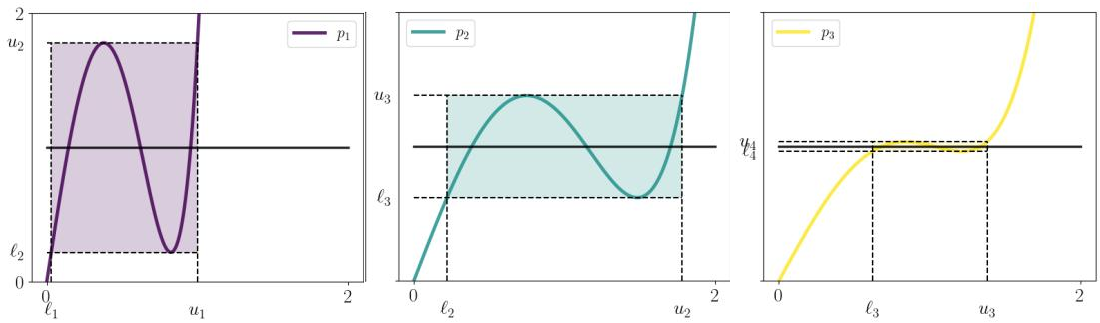
The evolution of the intervals shows how each polynomial narrows the range of singular values that still deviate from $1$1. The first polynomial maps the original singular value interval into a new interval closer to $1$1, the second polynomial acts on that updated interval, and subsequent polynomials continue refining the approximation. This interval-based view is what makes the greedy construction optimal for the spectral norm error.

To find each polynomial $p_t$pt​, the method solves a minimax approximation problem: among all odd polynomials of the chosen degree, it selects the one that uniformly approximates the constant function $1$1 on the current interval $[\ell_t,u_t]$[ℓt​,ut​]. For the low degrees used in practice, this can be done explicitly or with a simplified solver derived from the equioscillation property of minimax approximations. A full Remez-style procedure would also solve the problem, but because the target function is constant and the degree is small, the method uses a specialized low-degree construction that is simpler to implement and mathematically equivalent in the relevant setting.

The method also requires practical bounds on the singular values. A simple upper bound is $\|\boldsymbol M\|_{\mathrm F}$∥M∥F​, the Frobenius norm of the matrix. In practice, the input matrix is rescaled by a quantity proportional to this norm, and the upper bound is set to $u=1$u=1. The lower bound $\ell$ℓ is harder to estimate efficiently, so the authors choose a small value such as $\ell=10^{-3}$ℓ=10−3 for floating-point workloads, particularly when operating in bfloat16. A poor lower-bound estimate does not destroy convergence; it mainly delays it by a small number of iterations.

There are also numerical safeguards for finite-precision arithmetic. If roundoff causes singular values to appear slightly above the current upper bound, each polynomial can be replaced by $x\mapsto p_t(x/1.01)$x↦pt​(x/1.01), which effectively enlarges the interval and avoids instability. Because some optimal polynomials can be non-monotone near the beginning of the process, the early iterations can also use slightly suboptimal but less oscillatory polynomials. These changes stabilize the offline coefficient computation with negligible loss of approximation quality.

The overall pipeline has an offline stage and an online stage. During the offline stage, the polynomials $p_1,\dots,p_T$p1​,…,pT​ are precomputed once for fixed bounds $\ell$ℓ and $u$u. During the online stage, these stored coefficients are reused for every matrix update. For a degree-5 polynomial

the matrix iteration can be evaluated efficiently with a Horner-like form. Setting

the update is

In the recommended implementation, the composition is applied to a normalized matrix of the form

and a small number of iterations, typically five or six, are sufficient for the deep learning use case.

Experiment

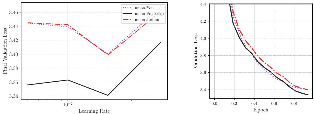
The experiments evaluate Polar Express both as an iterative polar-factor approximation and as the matrix sign subroutine in Muon, comparing it with Newton-Schulz, Jordan’s method, and You’s method. On synthetic and real matrix approximations, Polar Express converges more reliably and faster than the baselines when its lower singular value bound is reasonable, while remaining competitive when that bound is misestimated. In GPT-2 training, replacing these polar approximation subroutines with Polar Express consistently improves validation and training loss without extra cost, and ablations show that using only a few Polar Express iterations is sufficient, with further accuracy or exact SVD-based computation not helping optimization. The gains persist under weight decay and longer training, though the margin narrows.