One-sentence Summary

Researchers from Google, NYU, University of Montreal, and Facebook demonstrate that semantic information in deep networks resides in the representational space rather than in individual high-level units, and discover adversarial examples in which tiny imperceptible perturbations, found by maximizing the network's prediction error, cause misclassification and transfer across independently trained networks.

Key Contributions

• Unit analysis shows that individual high-level units cannot be distinguished from random linear combinations of high-level units, indicating that semantic information is encoded in the representation space rather than in isolated units.
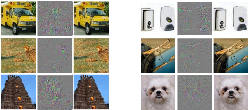
• An optimization procedure finds adversarial examples by producing barely perceptible perturbations that cause correctly classified images to be misclassified, demonstrating substantial discontinuities in deep-network input-output mappings near training examples.
• The same perturbation can cause a different network trained on a different dataset subset to misclassify the same input, indicating that adversarial perturbations are not random learning artifacts and supporting their use in constructive training schemes similar to hard-negative mining.

Introduction

Deep neural networks have become central to visual and speech recognition because they can learn complex mappings through many parallel nonlinear operations, and backpropagation makes this process effective in practice. However, their internal representations and decision boundaries are difficult to interpret, and prior work often assumed that individual neurons have clear semantic meanings and that tiny input changes should not affect classification. This work shows that these assumptions can fail: semantic information is better captured by the overall activation space than by specific units, and small, carefully chosen perturbations can create adversarial examples that flip predictions and transfer across models.

Method

The method is organized around three tightly connected ideas: inspecting individual activation units, constructing blind spot adversarial examples by nearest-image optimization, and measuring network instability through layerwise spectral bounds. Together, these components define a workflow for analyzing decision boundaries, identifying vulnerable regions in high-dimensional input space, and quantifying how small perturbations propagate through deep architectures.

The basic notation is that an image is represented as a vector $x \in \mathbb{R}^m$x∈Rm, while $\phi(x)$ϕ(x) denotes the activation values produced by a chosen hidden layer. The first analytical module treats hidden activations as candidate features and searches for images that strongly activate individual units. This follows a traditional feature inspection viewpoint: if a unit in $\phi(x)$ϕ(x) corresponds to an interpretable pattern, then one can search for inputs that maximize that unit’s response. Formally, for the $i$i-th coordinate of the activation space, the method examines inputs of the form

$$x' = \underset{x \in \mathcal{I}}{\arg\max}\ \langle \phi(x), e_i \rangle,$$x′=x∈Iargmax​ ⟨ϕ(x),ei​⟩,

where $e_i$ei​ is the basis vector selecting the $i$i-th activation coordinate and $\mathcal{I}$I denotes the space of valid images. This procedure produces visualizations that reveal which local stroke patterns, spatial configurations, or low-dimensional structure drive a particular unit. For handwritten digit models, such visualizations can isolate sensitivity to rounded strokes, diagonal segments, or upper or lower digit components.

For larger classifiers, the method treats the network as a label predictor

$$f:\mathbb{R}^m \rightarrow \{1,\ldots,k\},$$f:Rm→{1,…,k},

together with a continuous surrogate loss $\operatorname{loss}_f(x,l)$lossf​(x,l) for a target label $l$l. The central blind spot construction asks for the smallest additive perturbation $r$r that forces the classifier to assign image $x$x to a different label $l$l. This is formulated as a box-constrained nearest-image problem: minimize $\|r\|_2$∥r∥2​ subject to

$$f(x+r)=l,$$f(x+r)=l,

and

$$x+r \in [0,1]^m.$$x+r∈[0,1]m.

The resulting perturbed image is denoted $D(x,l)$D(x,l), representing a closest image to $x$x that $f$f classifies as $l$l. If $f(x)=l$f(x)=l, the problem is trivial, so the method focuses on the case $f(x)\neq l$f(x)=l. Because exact nearest decision-boundary computation is difficult for deep non-convex networks, the authors approximate $D(x,l)$D(x,l) using a box-constrained L-BFGS solver within a penalty-based framework. They find a sufficiently large scalar $c>0$c>0 such that the minimizer of

$$c\|r\|_2 + \operatorname{loss}_f(x+r,l)$$c∥r∥2​+lossf​(x+r,l)

satisfies the desired label constraint. The penalty term encourages small perturbations, while the loss term pushes the network toward the target class. For convex losses this would recover the exact nearest boundary point, but for neural networks it yields a practical approximation.

The architecture module supports the analysis across model families. For smaller digit models, the method examines fully connected networks with softmax output, as well as classifiers trained on top of an autoencoder. For natural image models, it examines deeper convolutional architectures, including standard supervised networks and very large unsupervised networks. The MNIST experiments also include weight decay regularization and optional splits of the training set into disjoint training and evaluation partitions, allowing the analysis to observe how perturbation behavior and unit sensitivity respond to changes in training constraints.

The final module analyzes instability through spectral properties of layers. If a network has $K$K layers, its activation map can be written as the composition

$$\phi(x)=\phi_K(\phi_{K-1}(\cdots \phi_1(x;W_1);W_2)\cdots;W_K),$$ϕ(x)=ϕK​(ϕK−1​(⋯ϕ1​(x;W1​);W2​)⋯;WK​),

where $\phi_k$ϕk​ maps layer $k-1$k−1 to layer $k$k using parameters $W_k$Wk​. The authors bound the additive stability of the whole network by the product of per-layer Lipschitz constants. For each layer, they define $L_k$Lk​ such that

$$\forall x,r,\quad \|\phi_k(x;W_k)-\phi_k(x+r;W_k)\|\le L_k\|r\|.$$∀x,r,∥ϕk​(x;Wk​)−ϕk​(x+r;Wk​)∥≤Lk​∥r∥.

The full network then satisfies

$$\|\phi(x)-\phi(x+r)\|\le L\|r\|,$$∥ϕ(x)−ϕ(x+r)∥≤L∥r∥,

with

$$L=\prod_{k=1}^K L_k.$$L=k=1∏K​Lk​.

Thus, adversarial sensitivity can be interpreted as amplification along the layerwise signal path. If early layers have large expansion factors, small input changes can produce large changes in later activations and ultimately in logits.

For a half-rectified layer, whether fully connected or convolutional, the mapping has the form

$$\phi_k(x;W_k,b_k)=\max(0,W_kx+b_k).$$ϕk​(x;Wk​,bk​)=max(0,Wk​x+bk​).

Because the rectifier $\rho(u)=\max(0,u)$ρ(u)=max(0,u) is contractive, the layer satisfies

$$\|\phi_k(x;W_k)-\phi_k(x+r;W_k)\|\le \|W_kr\|\le \|W_k\|\|r\|.$$∥ϕk​(x;Wk​)−ϕk​(x+r;Wk​)∥≤∥Wk​r∥≤∥Wk​∥∥r∥.

Therefore, a simple upper bound is

$$L_k\le \|W_k\|,$$Lk​≤∥Wk​∥,

where $\|W_k\|$∥Wk​∥ is the operator norm, namely the largest singular value. This gives a direct mechanism for estimating instability from learned weights.

The analysis also considers pooling and normalization. Max pooling is contractive because its Jacobian selects a subset of coordinates rather than expanding the input perturbation:

$$\forall x,r,\quad \|\phi_k(x)-\phi_k(x+r)\|\le \|r\|.$$∀x,r,∥ϕk​(x)−ϕk​(x+r)∥≤∥r∥.

For a contrast-normalization layer of the form

$$\phi_k(x)=\frac{x}{(\epsilon+\|x\|^2)^\gamma},$$ϕk​(x)=(ϵ+∥x∥2)γx​,

with $\gamma\in[0.5,1]$γ∈[0.5,1], the authors derive the bound

$$\forall x,r,\quad \|\phi_k(x)-\phi_k(x+r)\|\le \epsilon^{-\gamma}\|r\|.$$∀x,r,∥ϕk​(x)−ϕk​(x+r)∥≤ϵ−γ∥r∥.

This shows how normalization choices influence stability bounds.

For convolutional layers, the operator norm can be estimated spectrally. A convolution with $C$C input features, $D$D output features, spatial support $N\times N$N×N, and stride $\Delta$Δ can be written in terms of convolution kernels $w_{c,d}$wc,d​ as

$$Wx=\left\{\sum_{c=1}^C x_c\star w_{c,d}(n_1\Delta,n_2\Delta),\ d=1,\ldots,D\right\}.$$Wx={c=1∑C​xc​⋆wc,d​(n1​Δ,n2​Δ), d=1,…,D}.

Using Parseval’s formula, the operator norm becomes

$$\|W\|=\sup_{\xi\in[0,N\Delta^{-1})^2}\|A(\xi)\|,$$∥W∥=ξ∈[0,NΔ−1)2sup​∥A(ξ)∥,

where $A(\xi)$A(ξ) is a $D\times(C\cdot\Delta^2)$D×(C⋅Δ2) matrix whose $d$d-th row is

$$A(\xi)_d=\left(\Delta^{-2}\widehat{w_{c,d}}(\xi+l\cdot N\cdot\Delta^{-1}),\ c=1,\ldots,C,\ l=(0,\ldots,\Delta-1)^2\right).$$A(ξ)d​=(Δ−2wc,d​​(ξ+l⋅N⋅Δ−1), c=1,…,C, l=(0,…,Δ−1)2).

Here $\widehat{w_{c,d}}$wc,d​​ denotes the two-dimensional Fourier transform of kernel $w_{c,d}$wc,d​:

$$\widehat{w_{c,d}}(\xi)=\sum_{u\in[0,N)^2} w_{c,d}(u)e^{-2\pi i(u\cdot\xi)/N^2}.$$wc,d​​(ξ)=u∈[0,N)2∑​wc,d​(u)e−2πi(u⋅ξ)/N2.

This convolutional norm computation turns instability analysis into a spectral inspection of learned filters. Large operator norms in early layers indicate that the network can amplify small input perturbations, which is consistent with the existence of blind spot examples found by the optimization module. However, the bounds are conservative: a large bound does not by itself prove that an adversarial example exists, while a small bound indicates that no such example can occur under that Lipschitz measure. This observation motivates a regularization pathway in which upper Lipschitz bounds are penalized during training to reduce additive instability.

Experiment

Across MNIST, ImageNet, and a large YouTube image sample, the experiments examine activation patterns and adversarial behavior in fully connected, autoencoder, AlexNet, and QuocNet models. Random activation directions produce semantically meaningful images comparable to those from individual units, suggesting that networks do not clearly separate factors of variation along natural basis directions. Small, visually subtle perturbations consistently cause misclassification and often remain effective across different architectures, hyperparameters, and training sets, indicating that adversarial examples reflect general model blind spots rather than overfitting to one setting, while preliminary adversarial example augmentation appears to improve robustness. Spectral stability analysis shows that sensitivity can arise early in deep networks and suggests Lipschitz style regularization as a possible mitigation.

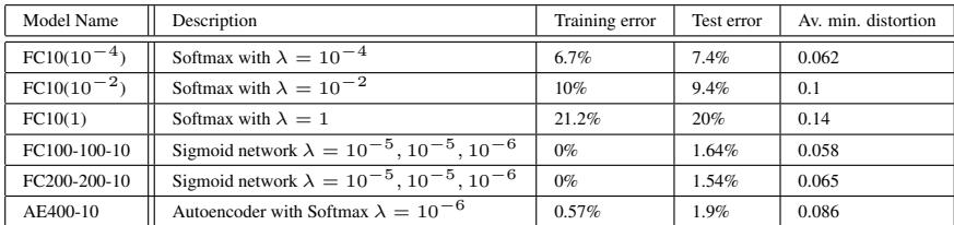
Across the MNIST models considered, adversarial examples can be generated with small average minimum distortion, and these low distortion perturbations occur for both simple softmax and deeper sigmoid or autoencoder models. Models with better test performance tend to show low distortion, while heavily regularized softmax variants have higher test error and larger distortion values. A relatively large fraction of adversarial examples is also reported to generalize across networks trained with different hyperparameters or on disjoint training sets. Many MNIST networks allow adversarial examples that are close to the original inputs, as measured by small average minimum distortion. Heavier softmax regularization coincides with worse test error and larger minimum distortion, while accurate sigmoid models retain low distortion.

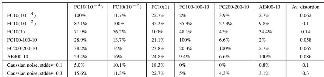
The results show that small adversarial distortions created for one network often cause misclassification in other networks trained with different architectures or hyperparameters, indicating cross-model generalization. The effect is strongest among fully connected variants and is more substantial than the impact of comparable random noise, while average distortion remains small. Adversarial examples generated for one model frequently transfer to models with different fully connected configurations. The transferred misclassification is more pronounced than Gaussian noise errors, suggesting structured distortions reveal shared blind spots. Average distortion values stay low, so the examples remain close to the original training data.

Evaluated fully connected models achieve low error on undistorted partitions and the common test set, while requiring only small average perturbation to create adversarial examples. The evidence indicates that such examples generalize across models with different layer sizes and even across models trained on disjoint partitions. Undistorted baseline errors remain low across the tested models Small average perturbations are enough to create adversarial examples Adversarial misclassification transfers across hyperparameter changes and disjoint training sets

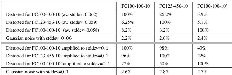
Adversarial perturbations generated for one fully connected network cause it to misclassify the targeted examples completely, while a smaller but noticeable fraction also fools other networks trained under different conditions. This cross-model effect is much stronger than random noise of a similar distortion size, and it becomes more pronounced when the perturbation is amplified. The results support the qualitative finding that small adversarial perturbations can generalize beyond the model that produced them. Adversarial examples are highly effective on the model for which they were generated. A nontrivial fraction of adversarial examples also cause errors on related networks trained from scratch with different hyperparameters or training data. Targeted adversarial perturbations produce much higher cross-model error than comparable Gaussian noise. Increasing the perturbation amplitude substantially strengthens the transferred misclassification effect.

The table reports upper bounds on the Lipschitz constants of rectified convolutional and fully connected layers in the network. These bounds are generally above one, indicating that small input perturbations can be amplified by the layerwise mapping. The bounds are conservative diagnostics, with large values suggesting possible unstability and small values providing a guarantee against such perturbations. Rectified convolutional and fully connected layers have upper Lipschitz bounds above one, indicating possible amplification of small perturbations. The first convolutional layer already has a bound greater than one, so instability can appear early in the network. Several convolutional layers have larger bounds than the fully connected layers, suggesting that convolutional stages can strongly contribute to unstability.

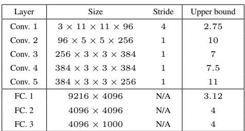
Experiments on MNIST classification models compare simple softmax, sigmoid, and autoencoder architectures, as well as fully connected and convolutional layers with Lipschitz diagnostics. The results show that accurately performing networks can be misled by very small input perturbations, and that these adversarial examples often transfer to models with different architectures, hyperparameters, or training sets. The transfer is much stronger than comparable random noise and grows with perturbation size, while Lipschitz bounds reveal that rectified layers can amplify small disturbances and introduce instability.