One-sentence Summary

Microsoft Research proposes Fast R-CNN, an object detection framework that employs several innovations to improve training and testing speed while increasing detection accuracy, training the VGG16 network $9\times$9× faster and testing $213\times$213× faster than R-CNN with higher mAP on PASCAL VOC 2012.

Key Contributions

• Fast R-CNN is introduced as a region-based ConvNet detector that uses a single-stage, multi-task training algorithm to update all network layers while jointly learning to classify object proposals and refine their spatial locations.
• The method eliminates disk-based feature caching and the multi-stage R-CNN pipeline, enabling faster and more efficient training and testing of very deep networks such as VGG16.
• On PASCAL VOC 2012, Fast R-CNN reaches 66% mAP, outperforms R-CNN, and is 9x faster than R-CNN in training and 213x faster at test time, with further gains over SPPnet in training speed, testing speed, and accuracy.

Introduction

Deep ConvNets have advanced image classification, but object detection is harder because it must both identify objects and localize them accurately. This requires processing many candidate object boxes, called proposals, and refining rough proposals into precise bounding boxes, which often hurts speed, accuracy, or training simplicity.

Prior detectors such as R-CNN and SPPnet achieved strong results but relied on multi-stage pipelines that separate feature extraction, classifier training, and bounding-box regression. These approaches were slow to train, required large feature caches on disk, and ran slowly at test time. SPPnet also could not fully update the convolutional layers, limiting accuracy for very deep networks.

The authors introduce Fast R-CNN, a single-stage training algorithm that jointly learns object classification and spatial bounding-box refinement using a multi-task loss. Their method updates all network layers, avoids feature caching, and is much faster to train than R-CNN and SPPnet while achieving higher detection accuracy on PASCAL VOC 2012.

Method

Fast R-CNN Architecture, Training, and Detection Pipeline

Fast R-CNN is formulated as a unified detection architecture that takes a full image and a set of object proposals as inputs, then jointly predicts class probabilities and refined bounding-box offsets for each proposal. The system first processes the entire image with a convolutional backbone composed of convolutional and max-pooling layers, producing a shared convolutional feature map. For each object proposal, a region of interest, or RoI, pooling layer extracts a fixed-length feature representation from this shared map. The resulting feature vector is passed through fully connected layers and split into two sibling branches: one branch produces softmax probabilities over object classes plus a background class, while the other branch predicts four real-valued bounding-box refinement offsets for each object class. Refer to the framework diagram

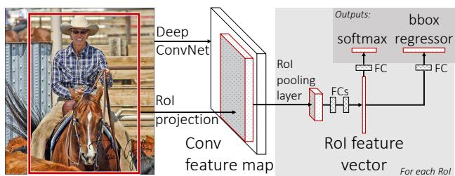
The RoI pooling layer is the central spatial interface between the convolutional backbone and the proposal-specific prediction heads. Each RoI is represented as a rectangular window in the convolutional feature map, defined by a tuple $(r, c, h, w)$(r,c,h,w), where $(r, c)$(r,c) is the top-left coordinate and $(h, w)$(h,w) is the height and width. RoI pooling divides this window into an $H \times W$H×W grid of sub-windows and applies max pooling inside each sub-window independently across feature channels. The output is a fixed-size $H \times W$H×W feature map, often chosen to match the spatial input expected by the first fully connected layer. For example, a VGG16-style configuration may use $H = W = 7$H=W=7. This mechanism allows proposals of different aspect ratios and sizes to be mapped to a common feature dimensionality while preserving the computational efficiency of a whole-image forward pass.

When adapting a pretrained ImageNet classification network for detection, the architecture undergoes three key transformations. First, the final max-pooling layer is replaced with a RoI pooling layer configured with the appropriate $H$H and $W$W values. Second, the final fully connected classification layer and softmax layer are replaced by two sibling output layers: a softmax classifier over $K+1$K+1 categories, including background, and a class-specific bounding-box regressor. Third, the input pipeline is modified to accept both an image list and an RoI list. These changes allow a standard image classification backbone to be repurposed as an end-to-end trainable detector.

Training Fast R-CNN is designed around hierarchical minibatch sampling to exploit feature sharing across proposals from the same image. Instead of treating every RoI as originating from a separate image, each stochastic gradient descent minibatch is formed by first sampling $N$N images and then sampling $R/N$R/N RoIs from each selected image. RoIs from the same image share the same convolutional forward pass and contribute to the same backward pass. This reduces redundant computation and memory usage substantially. For instance, with $N=2$N=2 and $R=128$R=128, two images contribute $64$64 RoIs each, making the training process far more efficient than sampling one RoI from each of $128$128 different images. The paper notes that this strategy can be roughly $64\times$64× faster than the R-CNN and SPPnet sampling approach.

Foreground and background RoIs are sampled according to their intersection-over-union overlap with ground-truth boxes. A portion of the RoIs, typically $25\%$25%, are sampled from proposals with IoU at least $0.5$0.5 and labeled with a foreground class $u \geq 1$u≥1. The remaining RoIs are sampled from proposals whose maximum IoU with ground truth lies in the interval $[0.1, 0.5)$[0.1,0.5) and are labeled as background with $u=0$u=0. The lower IoU threshold helps introduce hard background examples into training. Images are horizontally flipped during training with probability $0.5$0.5, but no additional augmentation is used.

The model is trained with a multi-task loss that jointly optimizes classification and localization. For each labeled RoI, let $p = (p_0, \ldots, p_K)$p=(p0​,…,pK​) denote the predicted softmax probability distribution over classes, $u$u the ground-truth class, $t^u$tu the predicted bounding-box regression offsets for class $u$u, and $v$v the ground-truth offsets. The total loss is

where the classification loss is the standard log loss

The localization term is only applied when the RoI is a foreground example. For background RoIs, $u=0$u=0 and the bounding-box regression loss is ignored. The localization loss is defined as

with

This smooth $L_1$L1​ loss is less sensitive to outliers than the $L_2$L2​ loss commonly used in earlier detection systems. It is especially useful for bounding-box regression because unbounded regression targets can otherwise lead to exploding gradients or require delicate learning-rate tuning. The hyperparameter $\lambda$λ controls the relative importance of localization, and the described setup uses $\lambda = 1$λ=1.

Backpropagation is routed through the RoI pooling layer by tracking the max-pooling argmax operations. If $y_{rj}$yrj​ is the output of RoI $r$r at pooled cell $j$j, and $x_i$xi​ is an input activation, then forward max pooling can be written as

During backward propagation, gradients are accumulated only through the input that attained the maximum in each sub-window:

This allows gradients from multiple RoIs to flow back into the shared convolutional layers, enabling true end-to-end fine-tuning of the entire detector.

For initialization, the fully connected output layers are set from Gaussian distributions with small standard deviations, biases are initialized to zero, and per-layer learning rates are scaled relative to the convolutional layers. Training uses momentum, parameter decay, and staged learning-rate reductions, but the core architectural contribution is the combination of shared image features, RoI pooling, hierarchical sampling, and a joint classification-localization objective.

Scale invariance can be handled in two ways. The first is brute-force learning, where images are processed at a fixed pixel size during both training and inference, forcing the network to learn scale variation directly from data. The second is image-pyramid training and inference, where each object proposal is approximately scale-normalized by assigning it to a pyramid level whose projected RoI area is close to a target size, such as $224^2$2242 pixels. During multi-scale training, a pyramid scale is randomly sampled when an image is selected, serving as a form of data augmentation.

At test time, detection reduces to a forward pass over an image, or an image pyramid, and a list of object proposals. For each proposal, the network outputs a softmax probability distribution and class-specific bounding-box offsets. The confidence for a given proposal and class $k$k is taken as the predicted probability $p_k$pk​, and non-maximum suppression is applied independently for each class to remove redundant detections.

A major runtime consideration is that detection requires processing many RoIs, so the fully connected layers can become a significant bottleneck despite their small cost in pure image classification. In a VGG16-style detector, the fully connected stages may consume nearly half of the forward-pass time when evaluating around $2000$2000 proposals. To address this, large fully connected layers can be compressed with truncated singular value decomposition. A weight matrix $W \in \mathbb{R}^{u \times v}$W∈Ru×v is approximated as

where $U$U contains the top $t$t left singular vectors, $\Sigma_t$Σt​ contains the top $t$t singular values, and $V$V contains the top $t$t right singular vectors. The original layer is replaced by two linear layers, one using $\Sigma_t V^T$Σt​VT and another using $U$U, without a nonlinearity between them. This changes the parameter count from $uv$uv to $t(u+v)$t(u+v) and can significantly reduce inference time when $t$t is much smaller than $\min(u, v)$min(u,v). As shown in the timing breakdown:

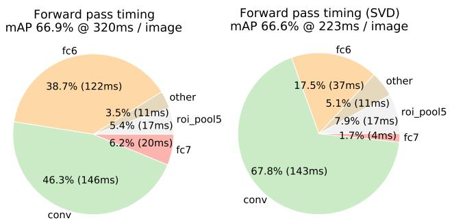
This compression strategy gives substantial speedups in the fully connected portion of the network with only a small loss in detection accuracy, making Fast R-CNN practical for systems that must score thousands of proposals per image.

Experiment

Experiments were conducted on PASCAL VOC benchmarks and preliminary MS COCO using three ImageNet-pretrained convolutional networks, with comparisons to R-CNN and SPPnet to assess detection accuracy, training and testing efficiency, and key design choices. The main results show that Fast R-CNN achieves strong detection performance while substantially reducing training and testing time, and that fine-tuning convolutional layers is especially important for very deep networks. Additional ablations validate that multi-task learning, single-scale processing, and expanded training data are beneficial, softmax can replace post-hoc SVMs, and adding excessive proposals can degrade accuracy rather than improve it.

The results compare Fast R-CNN with earlier detectors on VOC 2007 using VGG16. Fast R-CNN is competitive with R-CNN, improves when difficult examples are omitted from training, and gains further accuracy when VOC12 training images are added. The overall trend is that larger and cleaner training sets support better detection performance. Fast R-CNN trained on VOC07 exceeds R-CNN on several categories, including bird, boat, and person. Removing difficult examples from training increases Fast R-CNN overall average precision. Adding VOC12 training data further raises overall average precision and improves many individual classes.

On VOC 2010 test detection, Fast R-CNN is competitive with strong public leaderboard methods despite using mostly standard VGG16 training setups. SegDeepM slightly outperforms Fast R-CNN when extra segmentation annotations are used, while Fast R-CNN gains more from the enlarged union training set and moves ahead. The comparison also supports Fast R-CNN as a much faster alternative to methods based on the slower R-CNN pipeline. Fast R-CNN performs strongly across many object categories on VOC 2010. SegDeepM has a small overall edge over Fast R-CNN when trained with segmentation annotations. The enlarged 07++12 training set improves Fast R-CNN enough to surpass SegDeepM. Fast R-CNN is reported to run much faster than other tested R-CNN-based methods.

Fast R-CNN reaches the highest detection average precision among the compared methods on the benchmark. Using a larger training set further increases precision and strengthens the lead over prior results. The proposed detector gives the best overall average precision in the comparison. Training with the enlarged set improves detection performance over the smaller training configuration.

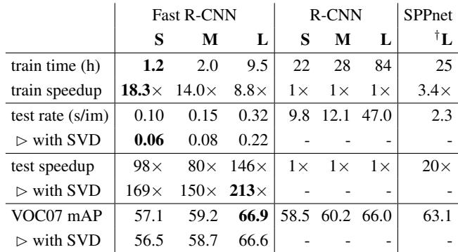
Fast R-CNN greatly reduces both training and testing runtime compared with R-CNN and SPPnet, with the largest speedups seen for the VGG16 model. Truncated SVD provides additional testing speedups while causing only a small accuracy loss. Fast R-CNN also avoids cached features, which removes a large disk storage requirement. Fast R-CNN trains and tests substantially faster than R-CNN and SPPnet. Truncated SVD further reduces detection time with only a slight mAP drop. Fast R-CNN avoids feature caching and therefore saves hundreds of gigabytes of disk storage.

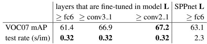
Restricting VGG16 fine-tuning to only fully connected layers reduces detection accuracy compared with fine-tuning deeper convolutional layers. Fine-tuning from conv3_1 and later recovers most of the accuracy while keeping the fast test rate, and extending to conv2_1 gives only a small gain while creating practical training constraints. Multi-scale SPPnet training shows a different accuracy speed tradeoff, with a much higher testing cost. Freezing the convolutional layers and training only the fully connected layers is not sufficient for VGG16 accuracy. Fine-tuning from conv3_1 and later is the practical choice, balancing accuracy and training cost. Extending fine-tuning to conv2_1 produces only a slight accuracy improvement and is less practical. Five-scale SPPnet training trades much slower evaluation for a different accuracy outcome.

Experiments on VOC 2007, VOC 2010, and related detection benchmarks evaluate Fast R-CNN against prior R-CNN-based detectors and show strong competitiveness, with overall detection accuracy improving when more training data is used or difficult examples are excluded. Runtime comparisons demonstrate that Fast R-CNN greatly accelerates both training and testing relative to R-CNN and SPPnet, avoids feature caching, and supports additional speedups from truncated SVD with only minor accuracy loss. Ablations on VGG16 fine-tuning indicate that training deeper convolutional layers is important, and fine-tuning from conv3_1 onward offers a practical accuracy and efficiency tradeoff, while multi-scale training increases computational cost.