One-sentence Summary

Researchers at LPENS, Université PSL, and Bocconi University demonstrate that diffusion models exhibit implicit dynamical regularization through two distinct timescales: an early $\tau_{\mathrm{gen}}$τgen​ at which high-quality samples emerge and a later $\tau_{\mathrm{mem}}$τmem​ growing linearly with dataset size $n$n beyond which memorization occurs, creating a widening generalization window that prevents overfitting even in highly overparameterized settings.

Key Contributions

• The study identifies two training timescales in diffusion models: τ_gen, when high-quality generation first emerges, and τ_mem, when memorization of training data begins.
• τ_mem grows linearly with training-set size n while τ_gen remains constant, creating a broader window for early stopping as n increases; memorization at long training times disappears only when n exceeds a model-dependent threshold.
• Numerical experiments with standard U-Net architectures on realistic and synthetic datasets and a tractable random-features analysis in the high-dimensional limit support the presence of an implicit dynamical regularization that can prevent memorization in highly overparameterized diffusion models.

Introduction

Diffusion models and score-based generative methods are now central for generating images, audio, video, and scientific data. They learn a score function that guides sampling from noise, but models trained to zero loss can recover the empirical score and memorize training examples. Prior work identified memorization in large models and studied regularizers such as architecture, learning rate, and early stopping, yet it remained unclear why highly expressive models often generalize before later overfitting.

The authors show that the training dynamics of score learning create an implicit regularization toward smooth, generalizing solutions. They identify two training timescales: an early time when high-quality novel samples emerge, and a much later time when the model begins memorizing the dataset. This second timescale grows with training set size, creating a wide early-stopping window for reliable generation.

Method

The authors leverage a compact score-learning model to isolate the architecture and training dynamics behind generalization and memorization in diffusion models. The core object is a score network parameterized as a two-layer Random Features Neural Network, where the first layer is random and frozen while the output layer is learned. For data in $\mathbb{R}^d$Rd, the score estimate is

$$\mathbf{s}_{\mathbf{A}}(\mathbf{x})=\frac{\mathbf{A}}{\sqrt{p}}\, \sigma\!\left(\frac{\mathbf{W}\mathbf{x}}{\sqrt{d}}\right),$$sA​(x)=p​A​σ(d​Wx​),

with $\mathbf{W}\in\mathbb{R}^{p\times d}$W∈Rp×d drawn from a Gaussian distribution and kept fixed, $\mathbf{A}\in\mathbb{R}^{d\times p}$A∈Rd×p updated during training, and $\sigma$σ applied elementwise. The analysis is carried out in the high-dimensional regime $d,p,n\to\infty$d,p,n→∞ while keeping

$$\psi_p=\frac{p}{d},\qquad \psi_n=\frac{n}{d}$$ψp​=dp​,ψn​=dn​

fixed. This parametrization provides a tractable score module: the nonlinear random features $\sigma(\mathbf{W}\mathbf{x}/\sqrt{d})$σ(Wx/d​) define a fixed nonlinear basis, and the learned matrix $\mathbf{A}$A controls how those features are combined into a vector field over the data space.

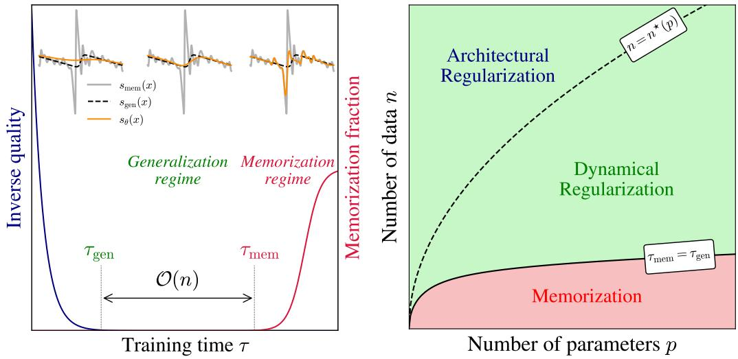
The overall learning trajectory, in which a model can first reach a generalization phase and later drift toward memorization, is summarized qualitatively in the framework illustration below.

The phase picture emphasizes two control knobs, the number of training points $n$n and the expressivity of the score model, often measured by the number of parameters $p$p. When $n$n is small, training can lead to memorization of the empirical score. As $n$n grows beyond a model-dependent threshold, the architecture itself prevents exact memorization, yielding what can be understood as architectural regularization. In addition, stopping training in an intermediate time window yields dynamical regularization, where the learned score is expressive enough to generalize but has not yet adapted fully to individual training samples.

The training pipeline is built around score matching at a fixed diffusion time $t$t. For a clean sample $\mathbf{x}$x and noise $\boldsymbol{\xi}\sim\mathcal{N}(0,\mathbf{I}_d)$ξ∼N(0,Id​), the noisy state is of the form

$$\mathbf{x}_t(\mathbf{x},\boldsymbol{\xi}) = e^{-t}\mathbf{x}+\sqrt{\Delta_t}\,\boldsymbol{\xi}.$$xt​(x,ξ)=e−tx+Δt​​ξ.

The empirical training objective is the score matching loss, rescaled by $1/d$1/d so that it remains finite as $d$d grows. Conceptually, the loss penalizes the score network when its output does not correctly undo the injected noise. The corresponding test loss and the distance to the population score are

$$\mathcal{L}_{\mathrm{test}} = \frac{1}{d}\mathbb{E}_{\mathbf{x},\boldsymbol{\xi}} \left[ \left\| \sqrt{\Delta_t}\,\mathbf{s}_{\mathbf{A}} (\mathbf{x}_t(\boldsymbol{\xi})) + \boldsymbol{\xi} \right\|^2 \right],$$Ltest​=d1​Ex,ξ​[​Δt​​sA​(xt​(ξ))+ξ​2],

and

$$\mathcal{E}_{\mathrm{score}} = \frac{1}{d} \mathbb{E}_{\mathbf{x}} \left[ \left\| \mathbf{s}_{\mathbf{A}}(\mathbf{x}) - \nabla \log P_{\mathbf{x}} \right\|^2 \right].$$Escore​=d1​Ex​[∥sA​(x)−∇logPx​∥2].

The first quantity measures in-sample and out-of-sample learning behavior, while the second measures how closely the learned field approaches the true population score. The gap

$$\mathcal{L}_{\mathrm{gen}} = \mathcal{L}_{\mathrm{test}} - \mathcal{L}_{\mathrm{train}}$$Lgen​=Ltest​−Ltrain​

is used as an indicator of overfitting.

The trainable output layer $\mathbf{A}$A is updated by gradient descent,

$$\mathbf{A}^{(k+1)} = \mathbf{A}^{(k)} - \eta\,\nabla_{\mathbf{A}} \mathcal{L}_{\mathrm{train}} (\mathbf{A}^{(k)}),$$A(k+1)=A(k)−η∇A​Ltrain​(A(k)),

where $\eta$η is the learning rate. In the small-learning-rate limit, and after rescaling discrete updates by

$$\tau=\frac{k\eta}{d^2},$$τ=d2kη​,

the discrete dynamics converges to a continuous gradient flow,

$$\dot{\mathbf{A}}(\tau) = - 2\Delta_t\frac{d}{p}\mathbf{A}\mathbf{U} - \frac{2d\sqrt{\Delta_t}}{\sqrt{p}}\mathbf{V}^T.$$A˙(τ)=−2Δt​pd​AU−p​2dΔt​​​VT.

The matrix $\mathbf{U}$U is the central object controlling the speed of learning. It is an empirical second-moment matrix of the random features under the noisy input distribution,

$$\mathbf{U} = \frac{1}{n} \sum_{\nu=1}^n \mathbb{E}_{\boldsymbol{\xi}} \left[ \sigma\!\left(\frac{\mathbf{W}\mathbf{x}_t^\nu(\boldsymbol{\xi})}{\sqrt{d}}\right) \sigma\!\left(\frac{\mathbf{W}\mathbf{x}_t^\nu(\boldsymbol{\xi})}{\sqrt{d}}\right)^T \right],$$U=n1​ν=1∑n​Eξ​[σ(d​Wxtν​(ξ)​)σ(d​Wxtν​(ξ)​)T],

and $\mathbf{V}$V contains correlations between the random features and the injected noise,

$$\mathbf{V} = \frac{1}{n} \sum_{\nu=1}^n \mathbb{E}_{\boldsymbol{\xi}} \left[ \sigma\!\left(\frac{\mathbf{W}\mathbf{x}_t^\nu(\boldsymbol{\xi})}{\sqrt{d}}\right) \boldsymbol{\xi}^T \right].$$V=n1​ν=1∑n​Eξ​[σ(d​Wxtν​(ξ)​)ξT].

Because the flow is linear in $\mathbf{A}$A, the dynamics can be solved exactly once the spectrum of $\mathbf{U}$U is known. The principal timescales of training are determined by the inverse eigenvalues of $\Delta_t\mathbf{U}/\psi_p$Δt​U/ψp​. Thus, the architecture design reduces the training-time behavior of score learning to a spectral analysis problem.

To analyze the spectrum, the method introduces diffusion-time dependent quantities $a_t$at​, $b_t$bt​, $v_t^2$vt2​, and $s_t^2$st2​ built from Gaussian expectations of the activation $\sigma$σ. These quantities capture how the nonlinearity mixes the data scale, the diffusion scale, and the frozen random projection. With these objects, the Stieltjes transform of the eigenvalue density of $\mathbf{U}$U satisfies a coupled system of equations. Once this system is solved, the density is recovered from the imaginary part of the Stieltjes transform.

In the strongly overparameterized regime, the spectrum separates into distinct components. When $\psi_p>\psi_n\gg1$ψp​>ψn​≫1, the spectral density can be written informally as

$$\rho(\lambda) = \left( 1-\frac{1+\psi_n}{\psi_p} \right) \delta(\lambda-s_t^2) + \frac{\psi_n}{\psi_p}\rho_1(\lambda) + \frac{1}{\psi_p}\rho_2(\lambda).$$ρ(λ)=(1−ψp​1+ψn​​)δ(λ−st2​)+ψp​ψn​​ρ1​(λ)+ψp​1​ρ2​(λ).

The atom proportional to $\delta(\lambda-s_t^2)$δ(λ−st2​) does not affect the training or test losses and can be ignored for the dynamics. The two remaining parts, $\rho_2$ρ2​ and $\rho_1$ρ1​, generate different timescales. The bulk $\rho_2$ρ2​ lives on the scale $\psi_p$ψp​, while $\rho_1$ρ1​ lives on the scale $\psi_p/\psi_n$ψp​/ψn​ when the model is strongly overparameterized. In the underparameterized regime $\psi_n>\psi_p\gg1$ψn​>ψp​≫1, the spectrum takes the form

$$\rho(\lambda) = \left( 1-\frac{1}{\psi_p} \right) \rho_1(\lambda) + \frac{1}{\psi_p}\rho_2(\lambda),$$ρ(λ)=(1−ψp​1​)ρ1​(λ)+ψp​1​ρ2​(λ),

again with $\rho_1$ρ1​ and $\rho_2$ρ2​ corresponding to distinct learning directions.

The bulk $\rho_2$ρ2​ is associated with the early generalization stage. Its eigenvalues produce a timescale $\tau_{\mathrm{gen}}$τgen​ of order $1/\Delta_t$1/Δt​. On this timescale, both training and test losses decrease, the generalization gap is effectively zero, and the model improves its approximation of the population score. The component $\rho_1$ρ1​ controls the later memorization stage. Its smaller eigenvalues produce a longer timescale,

$$\tau_{\mathrm{mem}} \sim \frac{\psi_p}{\Delta_t\lambda_{\min}},$$τmem​∼Δt​λmin​ψp​​,

where $\lambda_{\min}$λmin​ is the lower edge of the $\rho_1$ρ1​ bulk. In the overparameterized regime this becomes large and grows with the dataset size. On this longer timescale, the training loss continues to decrease, but the test loss begins to increase, reflecting overfitting to the finite sample score.

The dynamics predicted by this spectral analysis are visible directly in the Random Features training curves. Refer to the loss evolution figure below.

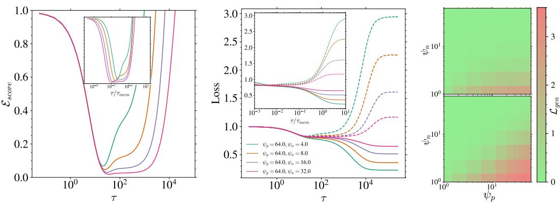
The trajectories show a fast decay of the distance to the true score followed by a later degradation. The test loss initially decreases along with the training loss, then increases after the memorization timescale is crossed. Rescaling time by $\tau_{\mathrm{mem}}$τmem​ collapses curves with different dataset sizes, confirming the spectral prediction that the second timescale is governed by the smallest relevant eigenvalues of the feature covariance. Heatmaps over $(\psi_n,\psi_p)$(ψn​,ψp​) further show how the generalization gap depends on the stopping time and on the parameter-to-data ratios.

For realistic diffusion models, the same training logic is studied with a conditional U-Net score architecture. The pipeline takes an image, applies the forward noise process, and feeds the noisy input together with a diffusion time embedding into the network. The score network uses three resolution levels with a base channel width $W$W and multipliers $1$1, $2$2, and $3$3, and a sinusoidal time embedding is added to the features at each resolution. Training proceeds with stochastic gradient descent using momentum, and the learned score is evaluated by generating samples and measuring both sample quality and memorization through nearest-neighbor comparisons.

The architecture-level behavior is shown below.

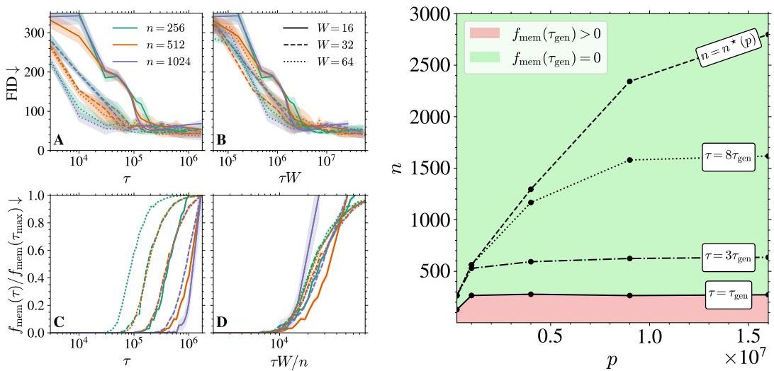
The curves illustrate how changing the number of parameters and the dataset size shifts the transition between generalization and memorization. When time is rescaled by the appropriate training-timescale factor, curves with different widths or dataset sizes align, indicating that the U-Net dynamics follows the same broad generalization-to-memorization structure identified in the Random Features analysis. The phase diagram also shows how the boundary between generalization and memorization moves with training time, reinforcing the dynamical regularization mechanism.

Experiment

Experiments trained diffusion models on grayscale CelebA images while varying dataset size and network capacity, tracking train and test losses, sample quality, and closeness to training examples to identify the shift from generalization to memorization. The results reveal a consistent two-phase training process: models first learn a reusable generative distribution, then later memorize the training set after a delayed overfitting stage, with larger datasets widening the useful early-training window and larger models compressing it. The study also shows that this behavior is not caused simply by repeated samples, but by the interaction of model expressivity, optimization time, and available data.