One-sentence Summary

Researchers at Harvard's Kempner Institute develop a random matrix theory framework that explains the striking consistency of diffusion models trained on non-overlapping data splits, formalizing finite-data effects through a self-consistent noise renormalization $\sigma^{2} \mapsto \kappa(\sigma^{2})$σ2↦κ(σ2) and identifying anisotropy, input inhomogeneity, and dataset-size scaling as spectral drivers of cross-split disagreement, with predictions validated on UNet and DiT architectures to establish a principled reproducibility baseline for generative training.

Key Contributions

• The work identifies shared Gaussian statistics and stable linear denoising maps as a concrete mechanism behind similar outputs from diffusion models trained on disjoint dataset splits with the same noise seed.
• A random matrix theory framework quantifies finite-data effects on the learned denoiser and sampling map in linear diffusion models, including self-consistent noise renormalization, eigenmode anisotropy, input inhomogeneity, and dataset-size scaling.
• The predictions are validated on linear diffusion models and on UNet and DiT architectures in the non-memorization regime, identifying spectral directions where cross-split samples deviate and establishing a reproducibility baseline for diffusion training.

Introduction

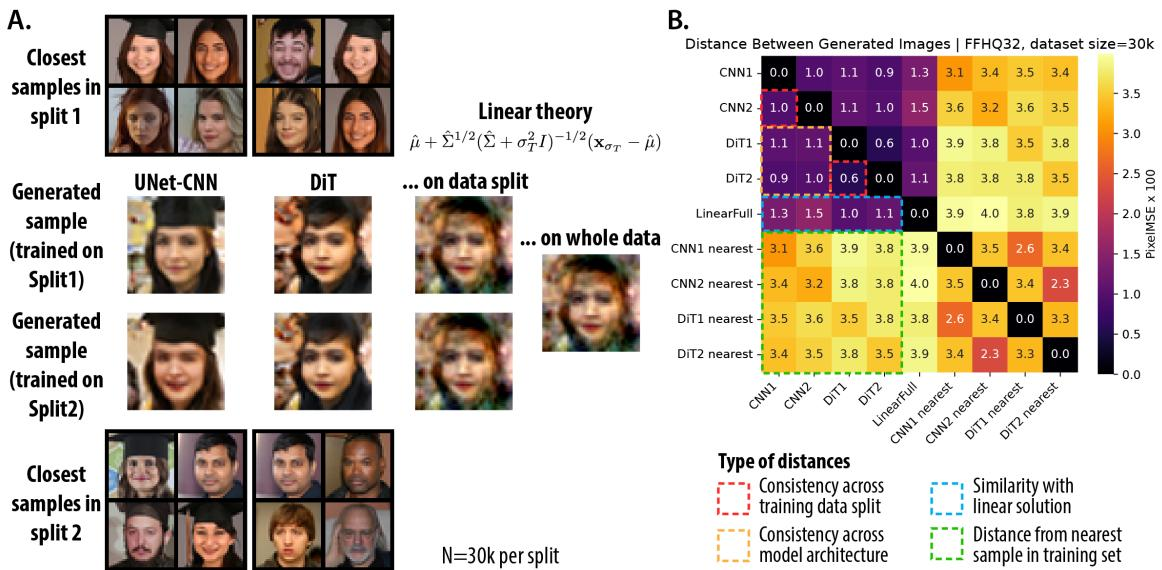
Diffusion models and flow matching now support generation in domains such as images, video, and proteins, and they show an unusual form of stability: independently trained models often map the same Gaussian noise seed to similar outputs. This run-to-run consistency matters because it suggests the learned vector fields capture stable statistical structure in the data, which affects claims about generalization, memorization, and creative variability. Prior work observed this phenomenon, but it lacked a clear finite-sample theory explaining why it occurs, while GANs and VAEs are complicated further by non-identifiable latent coordinates that can rotate across training runs. The authors leverage random matrix theory and a linear denoiser analysis to show that shared Gaussian statistics already predict cross-split agreement, and that finite data introduce deviations through a renormalized noise scale and a structured fluctuation law. They also extend deterministic equivalence to fractional matrix powers and validate the predicted effects in CNN and DiT diffusion models.

Method

The authors construct an analytical pipeline for studying how finite training data reshape score based diffusion models. The starting point is the EDM formulation, where a target data distribution $p_{0}(\mathbf{x})$p0​(x) is progressively blurred by Gaussian noise. For each noise scale $\sigma > 0$σ>0, the noised distribution is

$$p_{\sigma}(\mathbf{x}) = (p_{0} * \mathcal{N}(0,\sigma^{2}\mathbf{I}))(\mathbf{x}) = \int p_{0}(\mathbf{y}) \mathcal{N}(\mathbf{x} \mid \mathbf{y},\sigma^{2}\mathbf{I}) d\mathbf{y}.$$pσ​(x)=(p0​∗N(0,σ2I))(x)=∫p0​(y)N(x∣y,σ2I)dy.

The central object of the diffusion model is the score function $\nabla_{\mathbf{x}}\log p_{\sigma}(\mathbf{x})$∇x​logpσ​(x). Sampling is then described by the probability flow ODE

$$\frac{d\mathbf{x}}{d\sigma} = -\sigma \nabla_{\mathbf{x}}\log p_{\sigma}(\mathbf{x}).$$dσdx​=−σ∇x​logpσ​(x).

Integrating this trajectory from a large noise scale $\sigma_{T}$σT​ down to $\sigma = 0$σ=0 maps Gaussian noise to clean samples. In practice, the score is not learned directly. The authors first train a denoiser $\mathbf{D}_{\theta}$Dθ​ by minimizing the denoising score matching objective

$$\mathcal{L}_{\sigma} = \mathbb{E}_{\mathbf{x}_{0}\sim p_{0},\,\mathbf{z}\sim \mathcal{N}(0,\mathbf{I})} \left\| \mathbf{D}_{\theta}(\mathbf{x}_{0}+\sigma\mathbf{z};\sigma)-\mathbf{x}_{0} \right\|_{2}^{2}.$$Lσ​=Ex0​∼p0​,z∼N(0,I)​∥Dθ​(x0​+σz;σ)−x0​∥22​.

Once the denoiser is learned, Tweedie’s formula converts it into a score estimate,

$$\mathbf{s}_{\theta}(\mathbf{x},\sigma) = \frac{\mathbf{D}_{\theta}(\mathbf{x},\sigma)-\mathbf{x}}{\sigma^{2}}.$$sθ​(x,σ)=σ2Dθ​(x,σ)−x​.

Across practical diffusion training, the scale specific losses are combined through a weighting function $w(\sigma)$w(σ), giving an overall loss of the form

$$\mathcal{L} = \int_{\sigma} d\sigma\, w(\sigma)\mathcal{L}_{\sigma}.$$L=∫σ​dσw(σ)Lσ​.

This establishes the main training process: a neural denoiser is trained to remove Gaussian perturbations, and the trained denoiser is then converted into a score function that drives deterministic sampling.

To make the finite data behavior analytically tractable, the authors replace the neural denoiser with a linear affine denoiser at each noise scale,

$$\mathbf{D}(\mathbf{x};\sigma) = \mathbf{W}_{\sigma}\mathbf{x} + \mathbf{b}_{\sigma}.$$D(x;σ)=Wσ​x+bσ​.

In this setting, the learned denoiser depends on the training data only through its empirical mean and empirical covariance. Given an empirical covariance $\hat{\Sigma}$Σ^, the optimal linear denoiser is

$$\mathbf{D}_{\hat{\Sigma}}^{*}(\mathbf{x};\sigma) = \hat{\boldsymbol{\mu}} + (\hat{\boldsymbol{\Sigma}}+\sigma^{2}\mathbf{I})^{-1} \hat{\boldsymbol{\Sigma}} (\mathbf{x}-\hat{\boldsymbol{\mu}}).$$DΣ^∗​(x;σ)=μ^​+(Σ^+σ2I)−1Σ^(x−μ^​).

The authors isolate the effect of covariance fluctuation by fixing the mean and studying how random realizations of $\hat{\Sigma}$Σ^ alter denoiser outputs and final samples. They also identify the sampling map induced by the optimal linear denoiser. Starting from initial noise $\mathbf{x}_{\sigma_{T}}$xσT​​, the PF ODE gives the analytic trajectory

$$\mathbf{x}_{\hat{\boldsymbol{\Sigma}}}(\mathbf{x}_{\sigma_{T}},\sigma) = \hat{\boldsymbol{\mu}} + (\hat{\boldsymbol{\Sigma}}+\sigma^{2}\mathbf{I})^{1/2} (\hat{\boldsymbol{\Sigma}}+\sigma_{T}^{2}\mathbf{I})^{-1/2} (\mathbf{x}_{\sigma_{T}}-\hat{\boldsymbol{\mu}}).$$xΣ^​(xσT​​,σ)=μ^​+(Σ^+σ2I)1/2(Σ^+σT2​I)−1/2(xσT​​−μ^​).

Taking $\sigma \to 0$σ→0 recovers the final sampling map. Thus, in the linear case, the entire training and sampling process reduces to how the empirical covariance fluctuates across independent dataset realizations.

The core analytical tool used by the authors is deterministic equivalence. This method replaces random matrix expressions involving $\hat{\Sigma}$Σ^ with deterministic expressions involving the population covariance $\Sigma$Σ. The central replacement is

$$\hat{\boldsymbol{\Sigma}} (\hat{\boldsymbol{\Sigma}}+\lambda\mathbf{I})^{-1} \asymp \boldsymbol{\Sigma} (\boldsymbol{\Sigma}+\kappa(\lambda)\mathbf{I})^{-1},$$Σ^(Σ^+λI)−1≍Σ(Σ+κ(λ)I)−1,

where the scalar $\kappa(\lambda)$κ(λ) absorbs the stochastic effect of using finite samples. It is determined by the self consistent equation

$$\kappa(\lambda)-\lambda = \gamma \kappa(\lambda) \operatorname{tr} \left[ \boldsymbol{\Sigma} (\boldsymbol{\Sigma}+\kappa(\lambda)\mathbf{I})^{-1} \right], \qquad \gamma = d/n.$$κ(λ)−λ=γκ(λ)tr[Σ(Σ+κ(λ)I)−1],γ=d/n.

Here $d$d is the data dimension and $n$n is the number of samples. The mapping $\lambda \mapsto \kappa(\lambda)$λ↦κ(λ) can be interpreted as a renormalized noise scale. For trace like quantities, finite sample noise in $\hat{\Sigma}$Σ^ is replaced by an increased effective noise level in the population denoiser. This is analogous to a self energy correction, where randomness in the empirical covariance is integrated into a scalar correction term.

The authors use this machinery to compute the expected behavior of the denoiser across dataset realizations. For a fixed probe direction $\mathbf{v}$v, the expectation satisfies

$$\mathbb{E}_{\hat{\boldsymbol{\Sigma}}} \left[ \mathbf{v}^{\top} \mathbf{D}_{\hat{\boldsymbol{\Sigma}}}^{*}(\mathbf{x};\sigma) \right] \asymp \mathbf{v}^{\top} \left[ \boldsymbol{\mu} + \boldsymbol{\Sigma} (\boldsymbol{\Sigma}+\kappa(\sigma^{2})\mathbf{I})^{-1} (\mathbf{x}-\boldsymbol{\mu}) \right].$$EΣ^​[v⊤DΣ^∗​(x;σ)]≍v⊤[μ+Σ(Σ+κ(σ2)I)−1(x−μ)].

This result shows that finite data do not merely add noise to the denoiser. In expectation, they act by replacing the true noise scale $\sigma^{2}$σ2 with the renormalized scale $\kappa(\sigma^{2})$κ(σ2). Because $\kappa(\sigma^{2})$κ(σ2) is larger than $\sigma^{2}$σ2, the finite sample denoiser shrinks output components more aggressively, especially along low variance directions. This produces a bias toward the dataset mean, similar to adding an adaptive ridge penalty to the denoising objective.

The authors also derive the variance of the denoiser across independent training sets. They introduce the degrees of freedom functions

$$\operatorname{df}_{1}(\lambda) = \operatorname{Tr} \left[ \boldsymbol{\Sigma} (\boldsymbol{\Sigma}+\lambda\mathbf{I})^{-1} \right],$$df1​(λ)=Tr[Σ(Σ+λI)−1], $$\operatorname{df}_{2}(\lambda) = \operatorname{Tr} \left[ \boldsymbol{\Sigma}^{2} (\boldsymbol{\Sigma}+\lambda\mathbf{I})^{-2} \right],$$df2​(λ)=Tr[Σ2(Σ+λI)−2],

and

$$\operatorname{df}_{2}(\lambda,\lambda') = \operatorname{Tr} \left[ \boldsymbol{\Sigma}^{2} (\boldsymbol{\Sigma}+\lambda\mathbf{I})^{-1} (\boldsymbol{\Sigma}+\lambda'\mathbf{I})^{-1} \right].$$df2​(λ,λ′)=Tr[Σ2(Σ+λI)−1(Σ+λ′I)−1].

The variance of the linear denoiser output along direction $\mathbf{v}$v at input location $\mathbf{x}$x can be written as

$$\operatorname{Var}_{\hat{\boldsymbol{\Sigma}}} \left[ \mathbf{v}^{\top} \mathbf{D}_{\hat{\boldsymbol{\Sigma}}}^{*}(\mathbf{x};\sigma) \right] \asymp \frac{\kappa(\sigma^{2})^{2}} {n-\operatorname{df}_{2}(\kappa(\sigma^{2}))} \Diamond(\mathbf{v},\kappa(\sigma^{2}),\boldsymbol{\Sigma}) \Diamond(\mathbf{x}-\boldsymbol{\mu},\kappa(\sigma^{2}),\boldsymbol{\Sigma}),$$VarΣ^​[v⊤DΣ^∗​(x;σ)]≍n−df2​(κ(σ2))κ(σ2)2​◊(v,κ(σ2),Σ)◊(x−μ,κ(σ2),Σ),

where the spectral kernel is

$$\Diamond(\mathbf{u},\kappa,\boldsymbol{\Sigma}) = \mathbf{u}^{\top} (\boldsymbol{\Sigma}+\kappa\mathbf{I})^{-2} \boldsymbol{\Sigma} \mathbf{u}.$$◊(u,κ,Σ)=u⊤(Σ+κI)−2Σu.

This expression factorizes into three interpretable pieces. The first factor is a global scale controlled by sample size and effective noise. The second factor is an anisotropy term depending on the probe direction $\mathbf{v}$v. The third factor is an inhomogeneity term depending on the displacement of the input from the mean. When the probe direction aligns with an eigenvector of $\boldsymbol{\Sigma}$Σ with eigenvalue $\lambda_{k}$λk​, the anisotropy kernel reduces to a function that is maximized when $\lambda_{k}$λk​ is comparable to $\kappa(\sigma^{2})$κ(σ2). This means the largest denoiser disagreement occurs along modes whose data variance matches the renormalized noise scale.

The same perspective is extended from single step denoising to the full sampling map. For large terminal noise $\sigma_{T}$σT​, the linear sampling map is approximated by

$$\mathbf{x}_{\hat{\boldsymbol{\Sigma}}}(\mathbf{x}_{\sigma_{T}},0) = \boldsymbol{\mu} + \hat{\boldsymbol{\Sigma}}^{1/2} (\hat{\boldsymbol{\Sigma}}+\sigma_{T}^{2}\mathbf{I})^{-1/2} (\mathbf{x}_{\sigma_{T}}-\boldsymbol{\mu}) \approx \boldsymbol{\mu} + \hat{\boldsymbol{\Sigma}}^{1/2}\bar{\mathbf{x}},$$xΣ^​(xσT​​,0)=μ+Σ^1/2(Σ^+σT2​I)−1/2(xσT​​−μ)≈μ+Σ^1/2xˉ,

where

$$\bar{\mathbf{x}} = \frac{\mathbf{x}_{\sigma_{T}}-\boldsymbol{\mu}}{\sigma_{T}}.$$xˉ=σT​xσT​​−μ​.

The authors then use integral representations for fractional powers of covariance matrices to derive the expectation of the generated sample:

$$\mathbb{E}_{\hat{\boldsymbol{\Sigma}}} \left[ \mathbf{x}_{\hat{\boldsymbol{\Sigma}}}(\mathbf{x}_{\sigma_{T}},0) \right] \asymp \boldsymbol{\mu} + \frac{2}{\pi} \int_{0}^{\infty} \boldsymbol{\Sigma} (\boldsymbol{\Sigma}+\kappa(u^{2})\mathbf{I})^{-1} \bar{\mathbf{x}}\,du.$$EΣ^​[xΣ^​(xσT​​,0)]≍μ+π2​∫0∞​Σ(Σ+κ(u2)I)−1xˉdu.

Compared with the population sampling map, this expression integrates over a stronger shrinkage operator because $\kappa(u^{2}) > u^{2}$κ(u2)>u2. Therefore finite data produce systematic overshrinkage toward the mean, particularly along lower variance eigenmodes.

The variance of the final sample is expressed as a double integral over effective noise variables. With $\kappa = \kappa(u^{2})$κ=κ(u2) and $\kappa' = \kappa(v^{2})$κ′=κ(v2),

$$\operatorname{Var}_{\hat{\boldsymbol{\Sigma}}} \left[ \mathbf{v}^{\top} \mathbf{x}_{\hat{\boldsymbol{\Sigma}}}(\mathbf{x}_{\sigma_{T}},0) \right] \asymp \frac{4}{\pi^{2}} \int_{0}^{\infty} \int_{0}^{\infty} \frac{\kappa\kappa'} {n-\operatorname{df}_{2}(\kappa,\kappa')} \Diamond(\mathbf{v};\kappa,\kappa',\boldsymbol{\Sigma}) \Diamond(\bar{\mathbf{x}};\kappa,\kappa',\boldsymbol{\Sigma}) \,du\,dv,$$VarΣ^​[v⊤xΣ^​(xσT​​,0)]≍π24​∫0∞​∫0∞​n−df2​(κ,κ′)κκ′​◊(v;κ,κ′,Σ)◊(xˉ;κ,κ′,Σ)dudv,

where

$$\Diamond(\mathbf{a};\kappa,\kappa',\boldsymbol{\Sigma}) = \mathbf{a}^{\top} \boldsymbol{\Sigma} (\boldsymbol{\Sigma}+\kappa\mathbf{I})^{-1} (\boldsymbol{\Sigma}+\kappa'\mathbf{I})^{-1} \mathbf{a}.$$◊(a;κ,κ′,Σ)=a⊤Σ(Σ+κI)−1(Σ+κ′I)−1a.

Again, the variance factorizes into global scaling, probe direction anisotropy, and initial noise dependent inhomogeneity. The initial noise $\bar{\mathbf{x}}$xˉ acts as a spatial probe of the sampling map. Inputs whose deviations align strongly with high variance eigendirections experience larger cross split disagreement. Directionally, the variance is governed by the same spectral kernel, so the final sampling map inherits the spectral structure of the denoiser fluctuation.

The empirical validation of this analytical scheme is summarized below. As shown in the figure below:

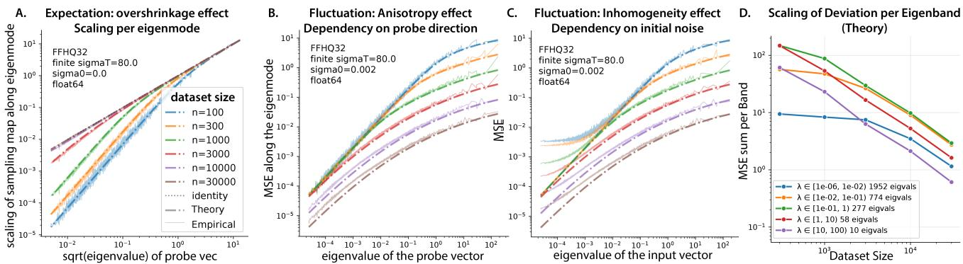
The curves compare theoretical deterministic equivalents with empirical linear diffusion computations for increasing dataset sizes. The expected scaling of the sampling map along eigenmodes shows overshrinkage toward the mean, with the strongest effect on low variance directions. The dependence of cross split mean squared error on probe eigenvalue shows that directional disagreement changes systematically across the spectrum, while the dependence on input eigenvalue shows that locations displaced along high variance modes induce larger uncertainty. The eigenband level scaling indicates that top eigenmodes can stabilize quickly with moderate data, whereas lower variance modes require substantially larger datasets before their cross split MSE decays.

Experiment

The experiments evaluate diffusion models trained on independent data splits and sampled with shared noise seeds, comparing UNet and DiT architectures, varying dataset sizes, and constructing statistically mismatched splits. These tests show that independently trained models often produce similar images, especially once training data are large enough to move beyond memorization, while deliberate mismatches in data means or variances disrupt this consistency. Numerical and network level validations further demonstrate that a Gaussian and random matrix theory framework predicts where samples vary across splits, with anisotropic and inhomogeneous deviations concentrated along data covariance eigendirections and requiring larger data sizes to resolve.