One-sentence Summary

This work proves the first rigorous quantitative bounds on grokking time in over-parameterized ridge regression trained with gradient descent and weight decay, demonstrating that grokking unfolds through overfitting, prolonged poor generalization, and eventual convergence, with the delay controllable through hyperparameter tuning rather than architectural changes and empirically validated on non-linear neural networks.

Key Contributions

• The paper proves end-to-end grokking in over-parameterized linear ridge regression trained with gradient descent and weight decay, including early overfitting, sustained poor generalization, and eventual arbitrarily small generalization error.

• The paper establishes quantitative bounds on the generalization delay, termed grokking time, in terms of training hyperparameters, and shows theoretically and empirically that proper hyperparameter tuning can amplify or eliminate grokking.

• The paper empirically shows that the derived bounds also capture grokking on nonlinear neural networks, and that a threshold-based accuracy metric recovers the familiar test error plateau in regression.

Introduction

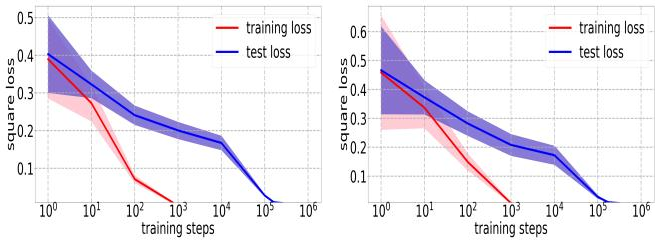
In deep learning and related ML systems, grokking is a counterintuitive overfitting phenomenon where training accuracy becomes perfect early, while test generalization improves only much later. This matters because it challenges standard regularization intuition and reveals hidden dynamics in how models converge during optimization. Prior theory often links grokking to regime changes in training, such as lazy-to-rich dynamics or weight-decay effects, but earlier analyses generally lack rigorous end-to-end guarantees, fail to prove that poor generalization persists long after overfitting, or study overly narrow settings. The authors leverage an over-parameterized linear ridge regression framework to provide the first provable end-to-end grokking result, showing that gradient descent can quickly fit the training data, maintain worse generalization for a quantifiable delay, and later converge to a well-generalizing global optimum, while also giving explicit hyperparameter bounds and demonstrating that weight decay can control the grokking time.

Method

The authors leverage a teacher-student regression pipeline to isolate the mechanism behind grokking. Each input $\pmb{x}_i \in \mathbb{R}^d$xi​∈Rd is sampled from a marginal distribution $\mathcal{D}_{\pmb{x}}$Dx​, and its label is given exactly by a fixed teacher function $N^*(\pmb{x})$N∗(x). The student model is linear in a feature representation:

$$N(\pmb{x};\pmb{\theta}) = \langle \pmb{\theta}, \phi(\pmb{x}) \rangle,$$N(x;θ)=⟨θ,ϕ(x)⟩,

where $\phi(\pmb{x}) : \mathbb{R}^d \mapsto \mathbb{R}^m$ϕ(x):Rd↦Rm is a fixed feature map and $\pmb{\theta} \in \mathbb{R}^m$θ∈Rm is trainable. The realizable assumption means that there exists some $\pmb{\theta}^*$θ∗ such that $N^*(\pmb{x}) = \langle \pmb{\theta}^*, \phi(\pmb{x}) \rangle$N∗(x)=⟨θ∗,ϕ(x)⟩.

Training is performed with ridge regression, which combines the empirical squared loss with an $\ell_2$ℓ2​ regularization term:

$$L_n(\pmb{\theta};\lambda) = \frac{1}{2n}\sum_{i=1}^n \left( \langle \pmb{\theta} - \pmb{\theta}^*, \phi(\pmb{x}_i) \rangle \right)^2 + \frac{\lambda}{2}\|\pmb{\theta}\|_2^2.$$Ln​(θ;λ)=2n1​i=1∑n​(⟨θ−θ∗,ϕ(xi​)⟩)2+2λ​∥θ∥22​.

The parameter is optimized using vanilla gradient descent:

$$\pmb{\theta}^{(t+1)} = \pmb{\theta}^{(t)} - \frac{\eta}{n} \sum_{i=1}^n \langle \pmb{\theta}^{(t)} - \pmb{\theta}^*, \phi(\pmb{x}_i) \rangle \phi(\pmb{x}_i) - \eta \lambda \pmb{\theta}^{(t)},$$θ(t+1)=θ(t)−nη​i=1∑n​⟨θ(t)−θ∗,ϕ(xi​)⟩ϕ(xi​)−ηλθ(t),

where $\eta$η is the learning rate and $\lambda$λ is the weight decay strength. The method studies training from a random initialization $\pmb{\theta}^{(0)} \sim \mathcal{N}(\pmb{0}, \nu^2 \pmb{I}_m)$θ(0)∼N(0,ν2Im​), which makes the early dynamics and the eventual decay of unused directions analytically tractable.

The central mechanism behind grokking is a subspace decomposition of the learned weights. Let $V = \operatorname{span}\{\phi(\pmb{x}_1),\ldots,\phi(\pmb{x}_n)\}$V=span{ϕ(x1​),…,ϕ(xn​)} denote the feature subspace spanned by the training examples. In the overparameterized regime $m \gg n$m≫n, the optimization can be understood by splitting $\pmb{\theta}$θ into a component $\pmb{\theta}_\parallel$θ∥​ inside $V$V and a component $\pmb{\theta}_\perp$θ⊥​ in the complementary subspace. The empirical gradient primarily updates $\pmb{\theta}_\parallel$θ∥​, allowing the model to fit the training data quickly. However, $\pmb{\theta}_\perp$θ⊥​ is invisible to the empirical loss and is mainly reduced by weight decay. Therefore, when $\lambda$λ is very small, training loss can decrease rapidly while the component responsible for poor population performance decays slowly.

This gives rise to two relevant time points. The first is

$$t_1 = \max\left(\left\{t \in \mathbb{N}: L_n(\pmb{\theta}^{(t)}) \geq \epsilon \right\}\right),$$t1​=max({t∈N:Ln​(θ(t))≥ϵ}),

which marks the end of rapid training loss reduction. The second is

$$t_2 = \min\left(\left\{t \in \mathbb{N}: L(\pmb{\theta}^{(t)}) \leq c \right\}\right),$$t2​=min({t∈N:L(θ(t))≤c}),

which marks the point where population loss becomes small. The authors show that, under sufficient sample size, large feature dimension, sufficiently small weight decay, and a compatible learning rate, $t_1$t1​ can be small while $t_2$t2​ can be arbitrarily large. Their bounds imply

$$t_1 \leq \frac{ n \ln\left( \frac{6b^2 \|\pmb{\theta}^{(0)}\|_2^2}{\epsilon} \right) }{ 2\eta \lambda_{\min}^+(\pmb{\Phi}^\top \pmb{\Phi}) },$$t1​≤2ηλmin+​(Φ⊤Φ)nln(ϵ6b2∥θ(0)∥22​​)​,

and

$$t_2 \geq \frac{ \ln\left( \frac{(m-n)\nu^2}{2} \left( \sqrt{\frac{c}{\lambda_{\min}(\pmb{\Sigma})}} + \|\pmb{\theta}^*\|_2 \right)^{-2} \right) }{ 4\eta \lambda },$$t2​≥4ηλln(2(m−n)ν2​(λmin​(Σ)c​​+∥θ∗∥2​)−2)​,

where $\pmb{\Phi}$Φ is the empirical feature matrix, $\pmb{\Sigma} = \mathbb{E}[\phi(\pmb{x})\phi(\pmb{x})^\top]$Σ=E[ϕ(x)ϕ(x)⊤] is the feature covariance matrix, and $b$b bounds the feature norm. These expressions make clear why a small $\lambda$λ can delay generalization without preventing fast training convergence.

To connect the theoretical bounds with observable hyperparameter behavior, the authors evaluate how $\lambda$λ, sample size $n$n, feature dimension $m$m, and initialization scale $\nu^2$ν2 change $t_1$t1​ and $t_2$t2​. As shown in the figure below:

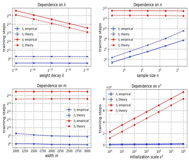
The plots indicate that decreasing $\lambda$λ primarily increases $t_2$t2​, because the orthogonal component $\pmb{\theta}_\perp$θ⊥​ decays more slowly under weak weight decay. Reducing $n$n can shorten $t_1$t1​ by making the training set easier to fit, thereby widening the interval $t_2 - t_1$t2​−t1​. Increasing $m$m has a comparatively muted effect in the plotted regime, while increasing $\nu^2$ν2 shifts both $t_1$t1​ and $t_2$t2​ upward at logarithmic rates, with $t_2$t2​ growing faster, which amplifies the grokking gap.

The empirical ridge regression pipeline uses the identity feature map in some experiments, so that the student predicts $\langle \pmb{\theta}, \pmb{x} \rangle$⟨θ,x⟩. Samples are generated under distributional assumptions on the features, often i.i.d. spherical Gaussian vectors, so that the covariance structure and the positive eigenvalue of the empirical Gram matrix can be estimated. The learning rate is fixed, and the model is trained by gradient descent with weight decay until both training and generalization behavior are observed.

The authors also extend the training protocol to a two-layer ReLU network. The network takes an input $\pmb{x} \in \mathbb{R}^d$x∈Rd, applies a first-layer weight matrix $\pmb{W}$W, passes the resulting hidden units through $\operatorname{ReLU}$ReLU, and combines them with a second-layer vector $\pmb{a}$a. The output has the form

$$N(\pmb{x};\pmb{W},\pmb{a}) = \sum_{j=1}^m a_j \operatorname{ReLU}\left(\langle \pmb{w}_j, \pmb{x} \rangle\right).$$N(x;W,a)=j=1∑m​aj​ReLU(⟨wj​,x⟩).

Both $\pmb{W}$W and $\pmb{a}$a are trained jointly with gradient descent and weight decay. The zero teacher is used as a simplified target, and the initialization scale $\nu^2$ν2 controls the initial norm of the first-layer weights. This nonlinear setup serves to check whether the same hyperparameter trends predicted by the ridge regression analysis appear beyond the linear feature model.

Experiment

The experiments use ridge regression and gradient descent with weight decay to empirically test the theoretical grokking behavior, comparing training and generalization error timelines under controlled hyperparameters. The results confirm that small weight decay can produce the predicted separation between early overfitting and later generalization, closely matching the theoretical bounds. Extensions to random-feature networks and fully trained nonlinear ReLU networks exhibit qualitatively similar grokking behavior, suggesting that the observed phenomenon is not limited to the idealized linear setting.