One-sentence Summary

Google DeepMind proposes specifying flexible, arbitrarily complex approximate posteriors in variational inference through normalizing flows built by applying sequences of invertible transformations to simple initial densities, unifying finite and infinitesimal flow categories and demonstrating improved inference quality when combined with amortized variational approaches.

Key Contributions

• Proposes specifying approximate posterior distributions in variational inference using normalizing flows, which transform a simple initial density through invertible mappings to learn complex non-Gaussian posteriors and yield a tighter modified variational lower bound with only linear-time additional terms.

• Develops finite and infinitesimal normalizing-flow categories, provides a unified view of related posterior approximation approaches as special flow types, and shows that infinitesimal flows are expressive enough in the asymptotic regime to recover the true posterior distribution.

• Demonstrates experimentally that amortized variational inference with general normalizing flows and efficient Monte Carlo gradient estimation systematically outperforms competing posterior approximation approaches on the evaluated problems, improving performance and applicability while retaining scalability.

Introduction

Variational inference is a core method for scalable probabilistic modeling, supporting large systems for text analysis, classification, image generation, and modeling of physical or chemical processes. Its practical power is limited by the choice of posterior approximation, because simple classes such as mean field distributions often cannot represent the true posterior and may underestimate uncertainty or bias parameter estimates. The authors leverage normalizing flows to construct flexible posterior approximations by transforming simple distributions through invertible mappings, yielding a tighter variational bound with low cost overhead and a class of approximations capable of recovering the true posterior in the asymptotic regime.

Method

The authors formulate variational inference as an optimization problem over an approximate posterior. For observations $\mathbf{x}$x, latent variables $\mathbf{z}$z, and model parameters $\theta$θ, the marginal likelihood requires integrating over $\mathbf{z}$z, which is generally intractable. Instead, they introduce a variational posterior $q_\phi(\mathbf{z}|\mathbf{x})$qϕ​(z∣x) and optimize a lower bound on the log marginal likelihood. The resulting bound is often written in terms of a free energy:

$$\mathcal{F}(\mathbf{x}) = \mathbb{E}_{q_\phi(\mathbf{z}|\mathbf{x})} \left[ \log q_\phi(\mathbf{z}|\mathbf{x}) - \log p_\theta(\mathbf{x},\mathbf{z}) \right].$$F(x)=Eqϕ​(z∣x)​[logqϕ​(z∣x)−logpθ​(x,z)].

Equivalently, the evidence lower bound is the negative of this free energy. It contains a reconstruction term and a regularization term that pushes the approximate posterior toward the prior.

The authors scale this optimization with minibatches and stochastic gradient estimation. For continuous latent variables, they use a reparameterization to compute gradients through sampling noise. If the variational posterior is Gaussian, then

$$\mathbf{z} = \boldsymbol{\mu} + \boldsymbol{\sigma}\boldsymbol{\epsilon}, \qquad \boldsymbol{\epsilon} \sim \mathcal{N}(\mathbf{0},\mathbf{I}),$$z=μ+σϵ,ϵ∼N(0,I),

where $\boldsymbol{\mu}$μ and $\boldsymbol{\sigma}$σ are produced by a neural network. This makes the sampling operation differentiable and allows standard backpropagation to estimate gradients of the expected log likelihood.

A central architectural module is the inference network. Rather than optimizing variational parameters separately for each data point, the model learns a global recognition network that maps observations directly to variational parameters. This amortizes inference, meaning the network generalizes across training and test data. The inference network is paired with a deep latent Gaussian generative model. The generative model contains a hierarchy of continuous latent variables,

$$p(\mathbf{x},\mathbf{z}_1,\dots,\mathbf{z}_L) = p\left(\mathbf{x}\mid f_0(\mathbf{z}_1)\right) \prod_{l=1}^{L} p\left(\mathbf{z}_l\mid f_l(\mathbf{z}_{l+1})\right),$$p(x,z1​,…,zL​)=p(x∣f0​(z1​))l=1∏L​p(zl​∣fl​(zl+1​)),

where the latent dependencies are specified by deterministic neural networks and the priors are standard Gaussians. The full system therefore behaves like an encoder decoder architecture: the inference network encodes observations into latent variables, and the generative network decodes those latent variables back into the observation space.

Refer to the framework diagram below:

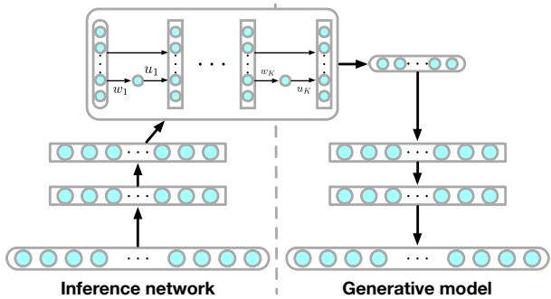
The left part of this system maps observations to the parameters of the variational approximation, while the right part represents the generative model that receives latent samples during training.

To improve the flexibility of the posterior approximation, the authors apply normalizing flows. A flow begins from a simple initial density, such as a Gaussian, and repeatedly applies invertible transformations. If the transformations are $f_1,\dots,f_K$f1​,…,fK​, then the final latent sample is

$$\mathbf{z}_K = f_K\circ f_{K-1}\circ \cdots \circ f_1(\mathbf{z}_0),$$zK​=fK​∘fK−1​∘⋯∘f1​(z0​),

and the transformed density is given by the change of variables rule:

$$\log q_K(\mathbf{z}_K) = \log q_0(\mathbf{z}_0) - \sum_{k=1}^{K} \log \left| \det \frac{\partial f_k}{\partial \mathbf{z}_k} \right|.$$logqK​(zK​)=logq0​(z0​)−k=1∑K​log​det∂zk​∂fk​​​.

This construction allows the variational posterior to become multimodal, skewed, or otherwise complex even when the base density is simple.

For scalable inference, the authors use transformations whose Jacobian determinants can be computed in linear time. One family is the planar flow,

$$f(\mathbf{z}) = \mathbf{z} + \mathbf{u}\,h(\mathbf{w}^{\top}\mathbf{z}+b),$$f(z)=z+uh(w⊤z+b),

where $h$h is a smooth nonlinearity and $\mathbf{w}$w, $\mathbf{u}$u, and $b$b are learnable parameters. The determinant is computed as

$$\det \left| \frac{\partial f}{\partial \mathbf{z}} \right| = \left| 1+\mathbf{u}^{\top}h'(\mathbf{w}^{\top}\mathbf{z}+b)\mathbf{w} \right|,$$det​∂z∂f​​=​1+u⊤h′(w⊤z+b)w​,

which requires only inner products and scales as $O(D)$O(D) for latent dimension $D$D. Planar flows expand or contract density around hyperplanes.

A second family is the radial flow,

$$f(\mathbf{z}) = \mathbf{z} + \beta h(\alpha,r)(\mathbf{z}-\mathbf{z}_0),$$f(z)=z+βh(α,r)(z−z0​),

where $r = \|\mathbf{z}-\mathbf{z}_0\|$r=∥z−z0​∥, $h(\alpha,r)=1/(\alpha+r)$h(α,r)=1/(α+r), and $\mathbf{z}_0$z0​, $\alpha$α, and $\beta$β are parameters. These maps expand or contract density around a reference point. Their determinants also admit closed form expressions with low computational cost. The transformations can be stacked to convert simple base densities into highly structured posteriors.

As shown in the figure below:

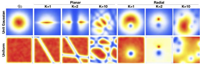
Simple initial densities can become elongated, multimodal, or spatially structured after one or more flow transformations.

The flow based posterior is optimized by rewriting the variational objective under the initial distribution. For a planar flow, the free energy can be evaluated as

$$\mathcal{F}(\mathbf{x}) = \mathbb{E}_{q_0(\mathbf{z}_0)} \left[ \log q_0(\mathbf{z}_0) - \log p_\theta(\mathbf{x},\mathbf{z}_K) - \sum_{k=1}^{K} \log \left| 1+\mathbf{u}_k^{\top} \boldsymbol{\psi}_k(\mathbf{z}_k) \right| \right].$$F(x)=Eq0​(z0​)​[logq0​(z0​)−logpθ​(x,zK​)−k=1∑K​log​1+uk⊤​ψk​(zk​)​].

In the amortized setting, the inference network outputs both the parameters of the base distribution $q_0$q0​ and the parameters of the flow transformations. During training, the system samples latent variables from the base density, passes them through the flow, evaluates the transformed latent density and the generative likelihood, and computes gradients with respect to both the generative model parameters $\theta$θ and the inference parameters $\phi$ϕ. Updates are performed with stochastic gradient methods using preconditioners that adapt the step size for each parameter. The overall cost combines the cost of the inference network with the cost of applying the flow and accumulating the log determinant terms, making the approach competitive with standard large scale variational inference systems.

Experiment

The experiments evaluate normalizing-flow posterior approximations in deep latent Gaussian models on synthetic two-dimensional densities and image datasets, using an annealed variational training objective. They show that flow-based approximations capture complex posterior structure, such as multimodality and periodicity, and that increasing flow length improves approximation quality. The results also indicate that learned planar flows are more parameter efficient than NICE and yield stronger posterior approximations and better likelihood-based model assessments.

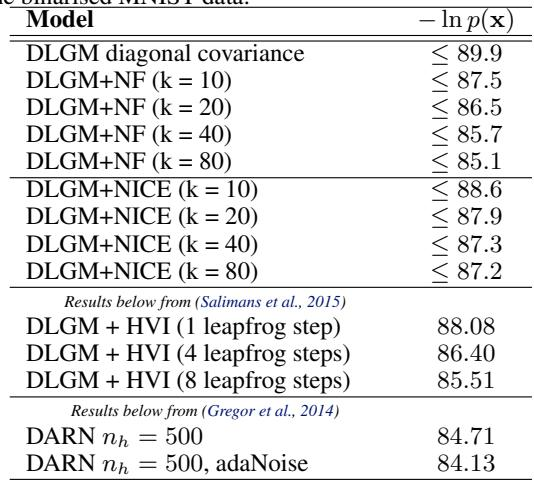
On binarized MNIST, using normalizing flow approximations within deep latent variable models reduces test negative log probabilities compared with a diagonal covariance baseline. Increasing the flow length gives a monotonic improvement for both flow families, and planar normalizing flows outperform NICE on comparable settings. Normalizing flow models achieve lower negative log probabilities than NICE volume preserving models. The diagonal covariance baseline has the weakest negative log probability among the listed entries. The best result is obtained with the normalizing flow at the largest tested flow length.

The comparison evaluates deep latent Gaussian models on CIFAR-10 patches using planar normalizing flows with different flow lengths. Increasing the flow length consistently improves the reported likelihood metric, supporting better posterior approximation. The results show that longer flows give better performance for the same model setup. Longer planar normalizing flow lengths systematically improve CIFAR-10 test performance. Improved test likelihoods indicate better approximate posteriors as flow length increases. The comparison holds the model setup fixed and varies only the flow length.

Experiments on binarized MNIST and CIFAR-10 patches evaluate deep latent variable models using normalizing flow approximations against baseline and volume-preserving alternatives. On MNIST, flow-based models provide better fit than the diagonal covariance baseline and NICE, with planar flows performing favorably and longer flows giving consistent gains. The CIFAR-10 comparison further shows that, for the same model setup, increasing planar flow length systematically improves test likelihood and posterior approximation.