One-sentence Summary

A residual learning framework reformulates layers as learning residual functions with reference to their inputs, enabling the training of networks up to 152 layers deep, $8\times$8× deeper than VGG nets with lower complexity, achieving $3.57\%$3.57% error on the ImageNet test set and winning first place on ILSVRC and COCO 2015 tasks.

Key Contributions

• A residual learning framework reformulates layers as learning residual functions relative to their inputs, enabling substantially deeper networks to be trained end-to-end with standard SGD and backpropagation without modifying the solvers.
• Experiments on ImageNet show that residual networks are easier to optimize and can gain accuracy with increased depth, with models up to 152 layers having lower complexity than VGG nets and an ensemble reaching 3.57% top-5 error and winning first place in the ILSVRC 2015 classification competition.
• Further validation on CIFAR-10 includes successfully trained models above 100 layers and exploration of models above 1000 layers, while deep residual representations produce a 28% relative improvement on COCO object detection and underpin first-place submissions on ImageNet detection, ImageNet localization, COCO detection, and COCO segmentation.

Introduction

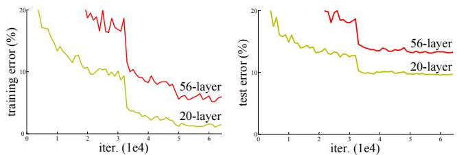
Deep convolutional neural networks transformed image classification and visual recognition because depth allows networks to integrate low, mid, and high level features, making very deep models important for strong performance. Although normalized initialization and intermediate normalization reduced vanishing and exploding gradient issues, the authors identify a degradation problem: deeper plain networks can show higher training error even without overfitting, indicating that current solvers struggle to optimize very deep networks directly. The authors address this by introducing residual learning, where stacked layers fit a residual mapping instead of an unreferenced mapping, using parameter free identity shortcut connections to make extremely deep networks easier to train and more accurate.

Method

Method

The authors leverage residual learning to make very deep convolutional networks easier to optimize. A key issue is that deeper plain networks can suffer from degradation: once the network is deep enough to converge, adding more layers may increase both training and test error even though the deeper model can represent the shallower one by adding identity mappings. The degradation is not simply a consequence of overfitting. It suggests that optimization solvers struggle to approximate identity mappings when they must be learned through multiple stacked nonlinear layers.

As shown in the figure below:

To address this, they reformulate the learning target. Let $\mathcal{H}(\mathbf{x})$H(x) denote the desired underlying mapping over a few stacked layers, with $\mathbf{x}$x being the input to those layers. Instead of forcing the layers to learn $\mathcal{H}(\mathbf{x})$H(x) directly, they let the layers learn a residual function

$$\mathcal{F}(\mathbf{x}) := \mathcal{H}(\mathbf{x}) - \mathbf{x},$$F(x):=H(x)−x,

so that the original mapping is reconstructed as

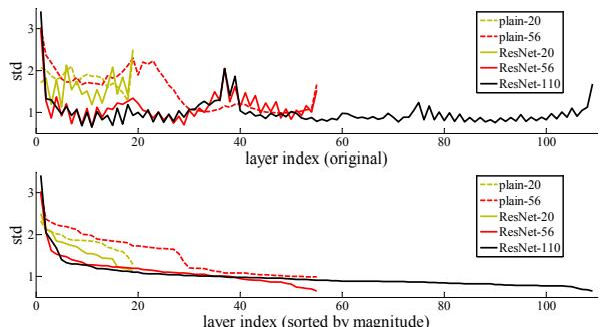
$$\mathcal{H}(\mathbf{x}) = \mathcal{F}(\mathbf{x}) + \mathbf{x}.$$H(x)=F(x)+x.

This reformulation makes identity mappings easier to approach: if the optimal mapping is close to identity, the residual function can simply be close to zero, and the solver can drive the weights toward small values. In practice, learned residual functions often have small magnitude, which supports the idea that identity mappings provide useful preconditioning for deep optimization.

As shown in the figure below:

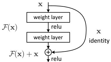
The residual formulation is implemented through shortcut connections. A basic building block is defined as

$$\mathbf{y} = \mathcal{F}(\mathbf{x}, \{W_i\}) + \mathbf{x},$$y=F(x,{Wi​})+x,

where $\mathbf{x}$x and $\mathbf{y}$y are the input and output of the block, and $\mathcal{F}(\mathbf{x}, \{W_i\})$F(x,{Wi​}) is the residual mapping learned by a few weighted layers. In a common two layer example, $\mathcal{F}$F can be written as $W_2 \sigma(W_1 \mathbf{x})$W2​σ(W1​x), where $\sigma$σ is a ReLU nonlinearity. The addition of $\mathbf{x}$x is performed through an identity shortcut, followed by another nonlinearity. This design does not add extra parameters or significant computation, allowing direct comparisons between plain and residual networks with the same depth, width, and computational budget.

The building block is shown in the figure below:

When the shortcut input and residual output have different dimensions, the identity mapping is no longer directly valid. In that case, the authors use a linear projection shortcut,

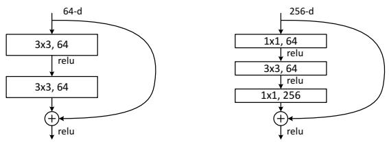
$$\mathbf{y} = \mathcal{F}(\mathbf{x}, \{W_i\}) + W_s \mathbf{x},$$y=F(x,{Wi​})+Ws​x,

typically implemented with $1 \times 1$1×1 convolutions when convolutional feature maps are used. They also show that the identity shortcut is generally sufficient for addressing degradation and is more economical, so projection shortcuts are mainly used for dimension matching. The form of $\mathcal{F}$F is flexible and may contain two or more convolutional layers. For deeper networks, a bottleneck design can compress the representation before a $3 \times 3$3×3 convolution and expand it again afterward, preserving the shortcut formulation while controlling computational cost.

A common residual function and bottleneck variant are shown in the figure below:

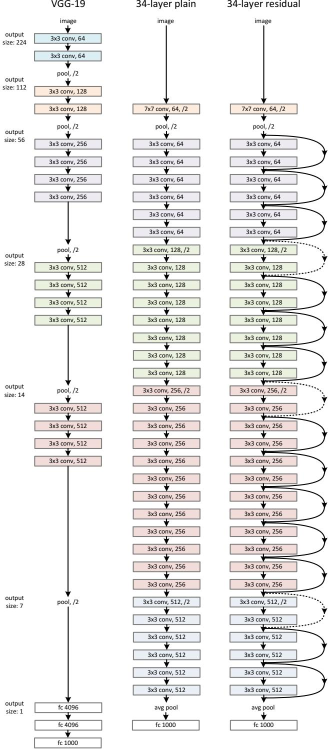
The overall architecture follows a plain deep convolutional design as the baseline, inspired by the philosophy of VGG style networks. It mainly uses $3 \times 3$3×3 convolutions and keeps the number of filters constant for a fixed feature map size. When the feature map resolution is halved, the number of filters is doubled to preserve per layer complexity. Downsampling is performed directly with strided convolutions, and the network ends with global average pooling followed by a fully connected softmax layer. The residual version keeps the same main layer stack and inserts shortcut connections around groups of layers. Solid line shortcuts denote identity mappings for equal dimensions, while dotted line shortcuts denote dimension changing paths, such as projection shortcuts or identity mappings with zero padding for increased channels.

Refer to the framework diagram below:

During training, images are randomly resized for scale augmentation, then cropped for training augmentation, and standard color augmentation is applied. Batch normalization is placed after each convolution and before activation. The networks are trained from scratch with stochastic gradient descent, using a mini batch size of 256. The initial learning rate is set to 0.1 and divided by 10 when the error plateaus. A weight decay of 0.0001 and momentum of 0.9 are used, while dropout is not applied. For testing, standard multi crop evaluation can be used, and for best performance the network is evaluated in a fully convolutional form and averaged over multiple input scales.

Experiment

Experiments on ImageNet, CIFAR-10, and detection benchmarks evaluate plain and residual networks to test whether residual learning alleviates optimization degradation in deep models. The results show that ordinary deeper networks are harder to train, whereas residual connections enable deeper models to converge and generalize better, with analyses indicating that residual functions typically have smaller responses. The learned representations also transfer strongly to object detection, demonstrating broad recognition improvements beyond classification.

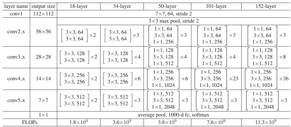
The table presents ImageNet architectures that share a common downsampling path and increase depth by stacking repeated building blocks. The shallower plain variants use paired 3x3 blocks, while the deeper variants use bottleneck blocks and place more repetitions in the high-dimensional stages. The cited experiments use these models for ImageNet classification and show that the deeper plain network suffers higher validation error than the shallower plain baseline. Model depth is expanded by repeating blocks while keeping the stage resolution pattern fixed. Plain architectures use stacked 3x3 block pairs, while deeper architectures use bottleneck block stacks. The deeper plain network performs worse than the shallower plain network despite having more capacity.

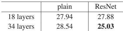
For ImageNet top-1 validation error, residual networks match or improve upon plain networks without adding parameters. Increasing depth from 18 to 34 layers hurts the plain network, but the residual network becomes markedly better. The result points to residual connections reducing degradation in deeper models. The 34 layer plain network performs worse than the 18 layer plain network. The residual network greatly improves the 34 layer model and matches the 18 layer model closely.

Residual networks improve over the 34-layer plain network on ImageNet validation in both top-1 and top-5 errors. Among the ResNet-34 variants, option C achieves the best errors, with option B slightly ahead of option A. The plain network trails the residual variants and remains less accurate than several reported baselines. Residual connections reduce validation error compared with the plain 34-layer network. Option C is the strongest of the three ResNet-34 variants. The evaluated models achieve competitive top-5 performance against prior ImageNet models.

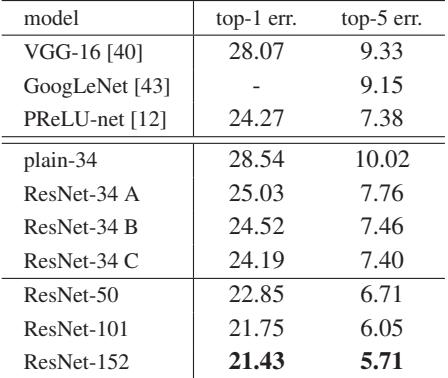
On the ImageNet results shown, ResNet-34 models achieve lower top-1 error than the compared VGG, PReLU, and BN inception baselines. The ResNet-34 C configuration has the best reported top-1 and top-5 errors among these rows, while VGG with top-1 accuracy is clearly less competitive. One VGG result is noted as being reported on the test set, unlike the other listed validation results. ResNet-34 improves ImageNet classification accuracy relative to the listed single-model baselines. The ResNet-34 C variant gives the strongest top-1 and top-5 performance among the reported rows.

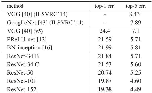
The comparison reports top-5 error rates for ensemble results on ImageNet, showing that earlier ILSVRC 2014 models have higher error than more recent approaches. Among the listed ensembles, ResNet shows the strongest test performance, while PReLU-net and BN-inception also reduce error relative to early VGG and GoogLeNet baselines. ResNet ensembles achieve the lowest reported top-5 error among the compared methods. More recent ensemble methods outperform the earlier ILSVRC 2014 VGG and GoogLeNet baselines.

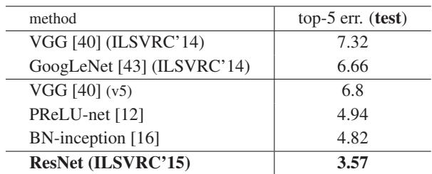
Experiments on ImageNet classification compare plain and residual architectures that share similar downsampling paths and grow depth through repeated blocks. The results show that simply deepening plain networks causes degradation, whereas residual connections allow deeper models to train more effectively and achieve better validation performance. Additional comparisons to prior baselines and ensembles indicate that the residual designs are more accurate than the plain network and competitive or stronger than representative deep-network methods.