One-sentence Summary

University of British Columbia and Amii propose a framework for analyzing the learning dynamics of LLM finetuning by decomposing how influence accumulates among candidate responses, yielding a unified interpretation of hallucination strengthening, the squeezing effect in off-policy DPO, and the advantages of on-policy DPO, and inspiring a simple method to improve alignment performance.

Key Contributions

• The paper develops a step-wise learning-dynamics framework for large language model finetuning that decomposes model prediction changes and unifies the analysis of instruction tuning, direct preference optimization and its variants, and reinforcement learning based methods.

• The framework explains counterintuitive finetuning behaviors, including strengthened hallucinations, repeated simple phrases in generated responses, and the squeezing effect that makes desired outputs less likely during off-policy direct preference optimization.

• Inspired by this analysis, the paper proposes a simple method for improving alignment performance and provides code for the experiments.

Introduction

Large language models are commonly aligned through instruction tuning and preference tuning so that they follow human directions and preferences more reliably. Prior analyses often focus on training objectives, endpoint behavior, or connections to reinforcement learning, but they explain less about how model predictions evolve step by step during finetuning. The authors leverage learning dynamics to derive a unified decomposition of how predictions change under supervised finetuning, DPO variants, and reinforcement learning based methods. Their framework explains counterintuitive behaviors such as repeating outputs, hallucination, and confidence decay in off-policy DPO, and they identify a squeezing effect from gradient ascent that motivates a simple method for better alignment.

Dataset

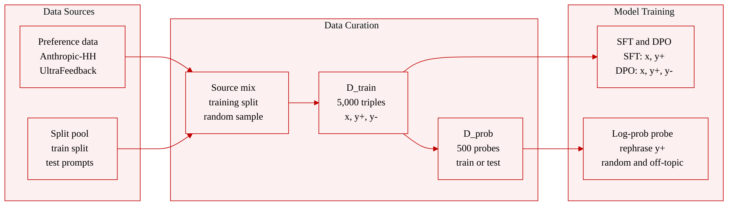
• The authors use two human preference datasets, Anthropic-HH and UltraFeedback, to build a small training subset for experimental analysis.

• The main training set, D_train, contains 5,000 examples randomly sampled from the training split. Each example has three components: a prompt or question x, a preferred response y+, and a less preferred response y-.

• The paper uses the data in two ways. For supervised fine-tuning, only x and y+ are used. For DPO-style learning, all three fields are used: x, y+, and y-.

• To study learning dynamics in more detail, the authors create a probing dataset, D_prob, by randomly sampling 500 examples from D_train.

• For each probing prompt x, they generate several additional response types to inspect how the model assigns probabilities over different outputs. These include a rephrasing of y+, an irrelevant response to another question x', and a randomly generated English sentence with the same word length as y+.

• In an appendix ablation, the authors also consider a probing variant where the prompts are taken from the test set.

• The probing set is used to examine changes in log-probabilities across response types over training, giving a finer view of how predictions evolve beyond the standard training examples.

Method

The authors leverage a learning dynamics framework that connects one gradient update on an update example $(\mathbf{x}_u,\mathbf{y}_u)$(xu​,yu​) to the change in predictions on an observing example $\mathbf{x}_o$xo​. For a model that produces logits $\mathbf{z}=h_\theta(\mathbf{x})$z=hθ​(x) and then applies softmax to obtain $\pi_\theta$πθ​, a gradient descent step with learning rate $\eta$η can be written as

$$\Delta \theta = -\eta \nabla_\theta \mathcal{L}\bigl(f_\theta(\mathbf{x}_u),\mathbf{y}_u\bigr).$$Δθ=−η∇θ​L(fθ​(xu​),yu​).

The framework tracks the resulting change in the model’s confidence on another input by measuring

$$\Delta \log \pi^t(\mathbf{y}\mid \mathbf{x}_o) \triangleq \log \pi_{\theta^{t+1}}(\mathbf{y}\mid \mathbf{x}_o) - \log \pi_{\theta^t}(\mathbf{y}\mid \mathbf{x}_o).$$Δlogπt(y∣xo​)≜logπθt+1​(y∣xo​)−logπθt​(y∣xo​).

For a single prediction vector, this per-step change decomposes into three interpretable factors:

$$\underbrace{\Delta \log \pi^t(\mathbf{y}\mid \mathbf{x}_o)}_{V\times 1} = -\eta \underbrace{\mathcal{A}^t(\mathbf{x}_o)}_{V\times V} \underbrace{\mathcal{K}^t(\mathbf{x}_o,\mathbf{x}_u)}_{V\times V} \underbrace{\mathcal{G}^t(\mathbf{x}_u,\mathbf{y}_u)}_{V\times 1} + \mathcal{O}(\eta^2).$$V×1Δlogπt(y∣xo​)​​=−ηV×VAt(xo​)​​V×VKt(xo​,xu​)​​V×1Gt(xu​,yu​)​​+O(η2).

Here,

$$\mathcal{A}^t(\mathbf{x}_o) = \nabla_{\mathbf{z}}\log \pi_{\theta^t}(\mathbf{y}\mid \mathbf{x}_o) = I-\mathbf{1}\pi_{\theta^t}^\top(\mathbf{x}_o),$$At(xo​)=∇z​logπθt​(y∣xo​)=I−1πθt⊤​(xo​),

so this term only depends on the current predictive distribution. The term

$$\mathcal{K}^t(\mathbf{x}_o,\mathbf{x}_u) = \nabla_\theta \mathbf{z}(\mathbf{x}_o)\, \nabla_\theta \mathbf{z}(\mathbf{x}_u)^\top$$Kt(xo​,xu​)=∇θ​z(xo​)∇θ​z(xu​)⊤

is the empirical neural tangent kernel of the logit network and acts as a model-specific local similarity between the update input and the observing input. The final term

$$\mathcal{G}^t(\mathbf{x}_u,\mathbf{y}_u) = \nabla_{\mathbf{z}}\mathcal{L}(\mathbf{x}_u,\mathbf{y}_u)$$Gt(xu​,yu​)=∇z​L(xu​,yu​)

is determined by the loss and supplies the direction and strength of the update. For cross entropy loss with a hard label, this term points from the current predicted distribution to the target one-hot distribution.

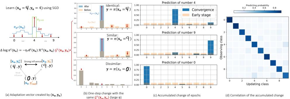
The analysis assumes that, during training, the relative influence of learning from $\mathbf{x}_u$xu​ on different observing inputs is reasonably stable. Under this assumption, the magnitude of $\mathcal{K}^t$Kt can be interpreted as a similarity signal. If $\|\mathcal{K}^t\|_F$∥Kt∥F​ is large, learning from $\mathbf{x}_u$xu​ is expected to influence the model’s prediction on $\mathbf{x}_o$xo​ strongly. If it is small, the influence is weak. Refer to the MNIST illustration below for this intuition: an update on one digit pulls up the probability of the same digit, indirectly increases the probability of similar digits from other classes, and has little effect on dissimilar inputs.

The same decomposition is extended to large language model finetuning by treating the prompt and response as one concatenated sequence. Let

$$\boldsymbol{\chi} = [\mathbf{x},\mathbf{y}],$$χ=[x,y],

where $\mathbf{y}=[y_1^+,\ldots,y_L^+]$y=[y1+​,…,yL+​] is a completion of length $L$L. The model outputs logits

$$\mathbf{z}=h_\theta(\boldsymbol{\chi}),$$z=hθ​(χ),

and each column of $\mathbf{z}$z is normalized by softmax to produce the conditional distribution over the next token. Causal masking ensures that the prediction of token $l$l does not use future tokens $y_{>l}$y>l​. With this construction, the empirical kernel becomes a tensor across token positions,

$$\mathcal{K}^t(\boldsymbol{\chi}_o,\boldsymbol{\chi}_u) \in \mathbb{R}^{V\times V\times L},$$Kt(χo​,χu​)∈RV×V×L,

and the change in the log probability of the $m$m-th observed token can be written as

$$\bigl[\Delta \log \pi^t(\mathbf{y}\mid \boldsymbol{\chi}_o)\bigr]_m = -\sum_{l=1}^{L} \eta \bigl[\mathcal{A}^t(\boldsymbol{\chi}_o)\bigr]_m \bigl[\mathcal{K}^t(\boldsymbol{\chi}_o,\boldsymbol{\chi}_u)\bigr]_l \bigl[\mathcal{G}^t(\boldsymbol{\chi}_u)\bigr]_l + \mathcal{O}(\eta^2).$$[Δlogπt(y∣χo​)]m​=−l=1∑L​η[At(χo​)]m​[Kt(χo​,χu​)]l​[Gt(χu​)]l​+O(η2).

For supervised finetuning, the loss is the negative log likelihood of the desired response:

$$\mathcal{L}_{\mathrm{SFT}}(\mathbf{x}_u,\mathbf{y}_u^+) = -\sum_{l=1}^{L} \log \pi(y=y_l^+\mid \mathbf{y}_{<l}^+,\mathbf{x}_u).$$LSFT​(xu​,yu+​)=−l=1∑L​logπ(y=yl+​∣y<l+​,xu​).

The corresponding residual term is roughly the difference between the model’s current predictive distribution and the target token distribution. Therefore, supervised finetuning creates an upward pressure on the desired response $\mathbf{y}_u^+$yu+​, a weaker indirect upward pressure on responses that are similar to $\mathbf{y}_u^+$yu+​ under the empirical kernel, and a downward pressure on the remaining probability mass because the distribution must sum to one. The SFT dynamics below illustrate how different response types move under these combined pressures.

Preference finetuning changes the geometry of the update because it introduces both positive and negative gradients. For direct preference optimization, the loss compares the chosen response $\mathbf{y}_u^+$yu+​ and the rejected response $\mathbf{y}_u^-$yu−​ relative to a reference policy $\pi_{\mathrm{ref}}$πref​:

$$\mathcal{L}_{\mathrm{DPO}}(\theta) = -\mathbb{E}_{(\mathbf{x}_u,\mathbf{y}_u^+,\mathbf{y}_u^-)\sim\mathcal{D}} \left[ \log \sigma \left( \beta \log \frac{ \pi_{\theta^t}(\mathbf{y}_u^+\mid \boldsymbol{\chi}_u^+) }{ \pi_{\mathrm{ref}}(\mathbf{y}_u^+\mid \boldsymbol{\chi}_u^+) } - \beta \log \frac{ \pi_{\theta^t}(\mathbf{y}_u^-\mid \boldsymbol{\chi}_u^-) }{ \pi_{\mathrm{ref}}(\mathbf{y}_u^-\mid \boldsymbol{\chi}_u^-) } \right) \right].$$LDPO​(θ)=−E(xu​,yu+​,yu−​)∼D​[logσ(βlogπref​(yu+​∣χu+​)πθt​(yu+​∣χu+​)​−βlogπref​(yu−​∣χu−​)πθt​(yu−​∣χu−​)​)].

Under teacher forcing, the per-step update can be decomposed into two competing terms:

$$\bigl[\Delta \log \pi^t(\mathbf{y}\mid \boldsymbol{\chi}_o)\bigr]_m = -\sum_{l=1}^{L} \eta \bigl[\mathcal{A}^t(\boldsymbol{\chi}_o)\bigr]_m \left( \bigl[\mathcal{K}^t(\boldsymbol{\chi}_o,\boldsymbol{\chi}_u^+)\bigr]_l \mathcal{G}_{\mathrm{DPO+}}^t - \bigl[\mathcal{K}^t(\boldsymbol{\chi}_o,\boldsymbol{\chi}_u^-)\bigr]_l \mathcal{G}_{\mathrm{DPO-}}^t \right) + \mathcal{O}(\eta^2).$$[Δlogπt(y∣χo​)]m​=−l=1∑L​η[At(χo​)]m​([Kt(χo​,χu+​)]l​GDPO+t​−[Kt(χo​,χu−​)]l​GDPO−t​)+O(η2).

The residual terms are

$$\mathcal{G}_{\mathrm{DPO+}}^t = \beta(1-a) \left( \pi_{\theta^t}(\mathbf{y}\mid \boldsymbol{\chi}_u^+) - \mathbf{y}_u^+ \right),$$GDPO+t​=β(1−a)(πθt​(y∣χu+​)−yu+​), $$\mathcal{G}_{\mathrm{DPO-}}^t = \beta(1-a) \left( \pi_{\theta^t}(\mathbf{y}\mid \boldsymbol{\chi}_u^-) - \mathbf{y}_u^- \right).$$GDPO−t​=β(1−a)(πθt​(y∣χu−​)−yu−​).

The scalar $a$a reflects how well the current policy already separates the chosen and rejected responses relative to the reference policy. As the margin grows, the update strength is automatically reduced. The coefficient $\beta$β controls the regularizing effect: a larger $\beta$β can strengthen the update when the model is behind the reference separation, but can also suppress the update when the model already achieves a positive margin. The diagram below summarizes the different updating vectors induced by supervised finetuning, direct preference optimization, and related preference methods.

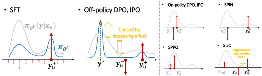
The key additional phenomenon introduced by preference finetuning is the squeezing effect. When a strong negative gradient is applied to a response $\mathbf{y}_u^-$yu−​ that has low probability under a peaked pretrained distribution, the softmax normalization redistributes the removed probability mass toward the output that was already most confident. Let

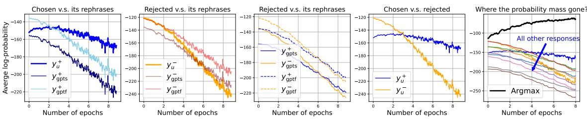
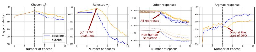
$$\mathbf{y}^* = \arg\max_{i\in[V]\setminus\{\mathbf{y}_u^-\}} \pi_{\theta^t}(\mathbf{y}=i).$$y∗=argi∈[V]∖{yu−​}max​πθt​(y=i).

Then the update guarantees that $\pi_{\theta^{t+1}}(\mathbf{y}=\mathbf{y}_u^-)$πθt+1​(y=yu−​) decreases, while a large portion of the removed mass is squeezed into $\pi_{\theta^{t+1}}(\mathbf{y}=\mathbf{y}^*)$πθt+1​(y=y∗). This produces a rich get richer pattern: high probability regions tend to increase, low probability regions tend to decrease, and a peakier initial distribution intensifies the effect. In practical preference finetuning, many tracked responses, including chosen responses, rejected responses, and rephrases, can all decay in log probability, while the probability mass accumulates in the current argmax or greedy decoded response. The off-policy DPO curves below make this probability mass flow visible.

Based on this mechanism, the authors propose an extended finetuning pipeline. Instead of performing supervised finetuning only on $[\mathbf{x}_u;\mathbf{y}_u^+]$[xu​;yu+​], the pipeline also trains on $[\mathbf{x}_u;\mathbf{y}_u^-]$[xu​;yu−​] during the supervised stage. This raises the likelihood of the rejected response and its local neighborhood before the preference optimization stage begins. Consequently, when direct preference optimization later applies a negative gradient to $\mathbf{y}_u^-$yu−​, that gradient acts on a more reasonable region of the distribution rather than on an extremely low-probability valley. The resulting supervised finetuning stage pulls up both the chosen and rejected regions, and the subsequent preference stage can push down the rejected response with a weaker squeezing effect. The learning dynamics below compare the baseline pipeline with this extended training design.

Experiment

The experiments use preference datasets and several small language models, alongside a probing dataset of representative responses, to examine how SFT and DPO update likelihoods over different response types. They confirm that SFT directly reinforces preferred responses while indirectly affecting similar responses, and that unrelated training targets can increase cross-question confidence, offering a mechanism for hallucination-like behavior. The DPO analysis shows that gradients on preferred and dispreferred responses propagate to neighboring responses and produce a growing preference margin, while also revealing a squeezing effect that can sharpen overly confident degenerate outputs. An augmented SFT stage that includes dispreferred responses mitigates this squeezing effect and leads to better generation quality after subsequent DPO training.

During DPO, the extended SFT pipeline becomes preferred over the baseline by both ChatGPT and Claude, despite starting with lower win rates before DPO. The improvement appears after DPO training, with the strongest advantage at an intermediate epoch and a later reduction that still leaves it ahead of the baseline. These results support the idea that including negative responses during SFT can mitigate the squeezing effect and improve final preference performance. The extended SFT pipeline starts behind the baseline in judge preferences before DPO. After DPO, it gains a consistent preference advantage against the baseline for both ChatGPT and Claude. The advantage is largest at an intermediate DPO epoch, then decreases but remains favorable.

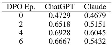
The experiments compare an extended SFT pipeline that includes negative responses against a baseline using preference judgments from ChatGPT and Claude during DPO. Although the extended pipeline is less preferred before DPO, it becomes consistently preferred after DPO, with its strongest advantage at an intermediate training epoch followed by a partial decline. These qualitative results suggest that incorporating negative responses during SFT can reduce the squeezing effect and lead to better final preference outcomes.