One-sentence Summary

Researchers at City University of Hong Kong, Tencent AI Lab, Xi'an Jiaotong University, and other institutions propose Variance Reduced Meta-CL (VR-MCL), which bridges Meta-Continual Learning with regularization-based methods by showing that Meta-CL implicitly performs online Hessian approximation and applying variance reduction to memory buffer sampling to achieve both timely and accurate Hessian estimation.

Key Contributions

• Meta-CL is connected to regularization-based continual learning by characterizing its hypergradients as online, implicit Hessian approximations, enabling timely second-order adaptation while exposing variance from random memory-buffer sampling.

• VR-MCL introduces a momentum-based hypergradient variance reduction technique that stabilizes online Hessian estimates, penalizing erroneous low-curvature updates and better preserving weights important for previous tasks.

• Theoretical analysis shows the variance reduction is equivalent to penalizing the implicitly estimated Hessian and provides a regret bound; experiments on three datasets and multiple continual-learning settings show consistent gains over state-of-the-art methods.

Introduction

Continual learning targets systems that learn sequentially from changing data streams while retaining earlier knowledge, making it important for real world adaptive models where standard i.i.d. supervised learning assumptions fail. Prior regularization methods preserve important parameters by estimating task importance through Hessian-based importance metrics, but those estimates are fixed after training and become less accurate as model parameters drift. Meta-continual learning uses memory buffer samples to update second-order information online through hypergradients, yet incomplete or biased memory sampling can introduce high variance and harmful Hessian estimates. The authors leverage Meta-CL’s online second-order perspective, connect it to regularization-based Hessian approximation, and propose Variance-Reduced Meta-CL, a momentum-based method that reduces hypergradient variance and acts as an implicit penalty on the estimated Hessian, helping suppress excessive updates and preserve previously learned knowledge with theoretical guarantees and empirical validation.

Method

The authors leverage a unified iterative update perspective to connect regularization-based continual learning, meta continual learning, and the proposed variance reduced algorithm. In continual learning, the model receives a sequence of tasks $\mathcal{T}^{1},\mathcal{T}^{2},\ldots,\mathcal{T}^{N}$T1,T2,…,TN, where the $i$i-th task contains samples $(\mathbf{x}_{n}^{i},y_{n}^{i})$(xni​,yni​). The ideal goal is to learn parameters $\theta$θ that minimize the average empirical risk over all observed tasks:

$$\min_{\theta}\frac{1}{j}\sum_{i=1}^{j}\mathcal{L}^{i}(\theta).$$θmin​j1​i=1∑j​Li(θ).

However, when the model trains on the current task $\mathcal{T}^{j}$Tj, it cannot directly access the original data of previous tasks $\mathcal{T}^{[1:j-1]}$T[1:j−1]. Regularization-based methods therefore approximate the previous-task risk instead of optimizing it directly. Using a second-order Taylor expansion around the parameters $\hat{\theta}^{i}$θ^i obtained after training on task $\mathcal{T}^{i}$Ti, the previous risk can be approximated by

$$\mathcal{L}_{j-1}^{\mathrm{prox}}(\theta) = \sum_{i=1}^{j-1} \underbrace{\mathcal{L}^{i}(\hat{\theta}^{i})}_{\text{constant term}} + \underbrace{(\theta-\hat{\theta}^{i})^{\top}\nabla_{\theta}\mathcal{L}^{i}(\hat{\theta}^{i})}_{\text{gradient term}} + \underbrace{\frac{1}{2}(\theta-\hat{\theta}^{i})^{\top}\mathbf{H}^{i}(\theta-\hat{\theta}^{i})}_{\text{Hessian term}},$$Lj−1prox​(θ)=i=1∑j−1​constant termLi(θ^i)​​+gradient term(θ−θ^i)⊤∇θ​Li(θ^i)​​+Hessian term21​(θ−θ^i)⊤Hi(θ−θ^i)​​,

where $\mathbf{H}^{i}=\nabla_{\theta}^{2}\mathcal{L}^{i}(\hat{\theta}^{i})$Hi=∇θ2​Li(θ^i) is the Hessian matrix for task $\mathcal{T}^{i}$Ti. The first term does not depend on $\theta$θ, and the gradient term is often near zero because each task is usually trained to convergence. Therefore, the most important approximation is the Hessian term. This leads to the unified regularized update rule

$$\theta \approx \theta - \alpha \left( \sum_{i=1}^{j-1}\mathbf{H}^{i} \right)^{-1} \nabla_{\theta}\mathcal{L}^{j}(\theta),$$θ≈θ−α(i=1∑j−1​Hi)−1∇θ​Lj(θ),

where $\alpha$α is the learning rate. In this update, directions with large Hessian curvature correspond to important weights for previous tasks. Multiplying the gradient by the inverse Hessian suppresses updates along those high-curvature directions, while allowing larger updates along low-curvature directions that are more compatible with the current task.

From this perspective, many regularization-based methods can be viewed as different Hessian approximation designs. For example, diagonal Fisher information matrices, diagonal importance estimates, and Kronecker factored approximations are all used to replace or approximate the accumulated Hessian. The central design principle is that better curvature estimation leads to a better tradeoff between stability on old tasks and plasticity on new tasks.

Meta continual learning reframes the same problem through bilevel optimization. Instead of explicitly storing or estimating individual task Hessians, it computes a hypergradient that propagates information from future inner-loop updates back to the current model parameters. Concretely, given a memory buffer $\mathcal{M}$M that stores samples from previous tasks, the method optimizes

$$\min_{\theta} \mathcal{L}^{[1:j]}(\theta_{(K)}) \quad \text{s.t.} \quad \theta_{(K)} = U_{K}(\theta;\mathcal{T}^{j}),$$θmin​L[1:j](θ(K)​)s.t.θ(K)​=UK​(θ;Tj),

where $U_{K}$UK​ denotes $K$K inner-loop update steps on the current task. One inner-loop step is written as

$$U(\theta_{(k)};\mathcal{T}_{(k)}^{j}) = \left[ \theta - \beta\nabla_{\theta}\mathcal{L}_{(k)}^{j}(\theta) \right]_{\theta=\theta_{(k-1)}},$$U(θ(k)​;T(k)j​)=[θ−β∇θ​L(k)j​(θ)]θ=θ(k−1)​​,

with $\beta$β as the inner-loop step size and $\mathcal{T}_{(k)}^{j}$T(k)j​ as a minibatch sampled from $\mathcal{T}^{j}$Tj.

The iterative update of Meta-CL can be separated into an inner loop and an outer loop. In the inner loop, the model starts from $\theta_{b(0)}=\theta_{b}$θb(0)​=θb​ and takes $K$K steps using samples from the current task, producing $\theta_{b(K)}$θb(K)​. In the outer loop, data $\epsilon_{b}$ϵb​ are sampled from the union of the current task and the memory buffer $\mathcal{M}$M, and the hypergradient with respect to the starting parameter $\theta_{b}$θb​ is computed as

$$\mathbf{g}_{\theta_{b}}^{\epsilon_{b}} = \frac{\partial \mathcal{L}(\theta_{b(K)};\epsilon_{b})}{\partial \theta_{b}}.$$gθb​ϵb​​=∂θb​∂L(θb(K)​;ϵb​)​.

The model is then updated by this hypergradient. As shown in the figure below:

The authors further show that, under a single inner-step simplification, Meta-CL also follows the same Hessian-style update rule:

$$\theta \approx \theta - \alpha (\mathbf{H}_{M}^{j})^{-1} \nabla_{\theta}\mathcal{L}^{j}(\theta).$$θ≈θ−α(HMj​)−1∇θ​Lj(θ).

Here, $\mathbf{H}_{M}^{j}$HMj​ is an implicit Hessian estimated from samples drawn from the memory buffer $\mathcal{M}$M. This gives Meta-CL an advantage over classic regularized methods because the Hessian information can be updated continuously rather than being fixed at the end of each previous task.

However, the same memory-based estimation introduces a vulnerability. If $\mathcal{M}$M does not contain enough representative samples from a previous task, the implicit Hessian may incorrectly assign low curvature to weights that are actually important for that task. In that case, the update is not sufficiently suppressed along those directions, causing forgetting. Therefore, reducing the variance of the hypergradient also reduces the variance of the implicitly estimated Hessian.

To address this issue, the authors propose Variance Reduced Meta Continual Learning, abbreviated as VR-MCL. Standard variance reduction methods such as SAG, SAGA, and SVRG require full-batch gradients over all samples in a task, which is difficult in online continual learning because data arrive in minibatches and the full task set may never be visible. VR-MCL instead uses a momentum-based variance reduction design. At outer iteration $b$b, it retains the momentum component from the previous iteration and reuses the current outer-loop data to evaluate a correction term.

The update flow for the $b$b-th iteration is shown in the figure below:

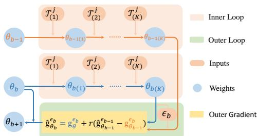
In this framework, $\hat{\mathbf{g}}_{\theta_{b-1}}^{\epsilon_{b-1}}$g^​θb−1​ϵb−1​​ stores the reduced gradient from the previous outer step, $\mathbf{g}_{\theta_{b-1}}^{\epsilon_{b}}$gθb−1​ϵb​​ denotes the hypergradient evaluated on the previous parameter trajectory using the current outer data $\epsilon_{b}$ϵb​, and $\mathbf{g}_{\theta_{b}}^{\epsilon_{b}}$gθb​ϵb​​ denotes the hypergradient evaluated on the current parameter trajectory. The variance-reduced update gradient is

$$\hat{\mathbf{g}}_{\theta_{b}}^{\epsilon_{b}} = \mathbf{g}_{\theta_{b}}^{\epsilon_{b}} + r \left( \hat{\mathbf{g}}_{\theta_{b-1}}^{\epsilon_{b-1}} - \mathbf{g}_{\theta_{b-1}}^{\epsilon_{b}} \right),$$g^​θb​ϵb​​=gθb​ϵb​​+r(g^​θb−1​ϵb−1​​−gθb−1​ϵb​​),

where $r$r is the momentum ratio. This update uses the difference between a stored previous reduced gradient and a newly computed hypergradient at the previous parameter to correct sampling noise. The final model parameter can then be updated by

$$\theta_{b+1} = \theta_{b} - \alpha \hat{\mathbf{g}}_{\theta_{b}}^{\epsilon_{b}}.$$θb+1​=θb​−αg^​θb​ϵb​​.

The variance reduction analysis examines the difference between the estimated gradient and the unknown full-batch gradient direction. Let

$$\Delta_{b} = \hat{\mathbf{g}}_{\theta_{b}}^{\epsilon_{b}} - \mathrm{G}_{\theta_{b}},$$Δb​=g^​θb​ϵb​​−Gθb​​,

where $\mathrm{G}_{\theta_{b}}$Gθb​​ denotes the true full-batch gradient direction at $\theta_{b}$θb​. Substituting the VR-MCL update gives

$$\Delta_{b} = r\Delta_{b-1} + (1-r) \left( \mathbf{g}_{\theta_{b}}^{\epsilon_{b}} - \mathrm{G}_{\theta_{b}} \right) + r \left( \mathbf{g}_{\theta_{b}}^{\epsilon_{b}} - \mathbf{g}_{\theta_{b-1}}^{\epsilon_{b}} - \left( \mathrm{G}_{\theta_{b}} - \mathrm{G}_{\theta_{b-1}} \right) \right).$$Δb​=rΔb−1​+(1−r)(gθb​ϵb​​−Gθb​​)+r(gθb​ϵb​​−gθb−1​ϵb​​−(Gθb​​−Gθb−1​​)).

The second term can be controlled through $r$r, while the third term is expected to be small when the parameter change between successive iterations is small. Thus, the estimator error remains bounded and can be driven toward a smaller residual, which explains the variance-reduction effect.

From the Hessian perspective, the variance-reduced gradient update is equivalent to modifying the inverse implicit Hessian used in Meta-CL. Specifically, the VR-MCL update can be written as

$$\theta \approx \theta - \alpha (\mathbf{H}_{\mathrm{VR}}^{j})^{-1} \nabla_{\theta}\mathcal{L}^{j}(\theta),$$θ≈θ−α(HVRj​)−1∇θ​Lj(θ),

where the reduced inverse Hessian has the approximate form

$$(\mathbf{H}_{\mathrm{VR}}^{j})^{-1} = (\mathbf{H}_{M_{b}}^{j})^{-1} + r \left( (\widehat{\mathbf{H}}_{M_{b-1}}^{j})^{-1} - (\overline{\mathbf{H}}_{M_{b-1}}^{j})^{-1} \right).$$(HVRj​)−1=(HMb​j​)−1+r((HMb−1​j​)−1−(HMb−1​j​)−1).

Here, $\mathbf{H}_{M_{b}}^{j}$HMb​j​ is the current Hessian approximation computed from outer-loop data $\epsilon_{b}$ϵb​, $\widehat{\mathbf{H}}_{M_{b-1}}^{j}$HMb−1​j​ corresponds to the Hessian information carried by the momentum term from the previous step, and $\overline{\mathbf{H}}_{M_{b-1}}^{j}$HMb−1​j​ corresponds to the Hessian evaluated at the previous parameter using the current data.

This formula shows that VR-MCL acts like a regularizer on the implicit Hessian. If Meta-CL wrongly estimates a direction as low curvature because of insufficient memory samples, the correction term can reduce the inverse curvature in that direction. In eigenvalue notation, when a previously important weight is incorrectly assigned a very small curvature $v_{b}$vb​ but the momentum term implies much larger curvature $\hat{v}_{b-1}$v^b−1​, the adjusted inverse curvature becomes approximately

$$v_{b}^{-1} + r \left( (\hat{v}_{b-1})^{-1} - (\overline{v}_{b-1})^{-1} \right) \le v_{b}^{-1}.$$vb−1​+r((v^b−1​)−1−(vb−1​)−1)≤vb−1​.

This makes the update smaller along directions that may actually store important old-task knowledge. Conversely, when the Hessian eigenvalues are already consistent across the current and previous estimates, the correction term is close to zero, so the update remains cautious along high-curvature directions. In this way, the algorithm treats variance reduction as curvature stabilization.

Under assumptions of smoothness, boundedness, and strong convexity in a stochastic online setting, the authors also derive a regret bound of the form

$$\mathbf{CR}_{j} = \widetilde{\mathcal{O}}(\sqrt{T}),$$CRj​=O(T​),

where $T$T is the number of training iterations and $\mathbf{CR}_{j}$CRj​ measures the gap between the accumulated loss of the learned model and the best fixed model for the observed tasks. This bound supports the effectiveness of the proposed training process by showing that reduced hypergradient variance can lead to nearly optimal regret behavior in the online continual learning formulation.

Experiment

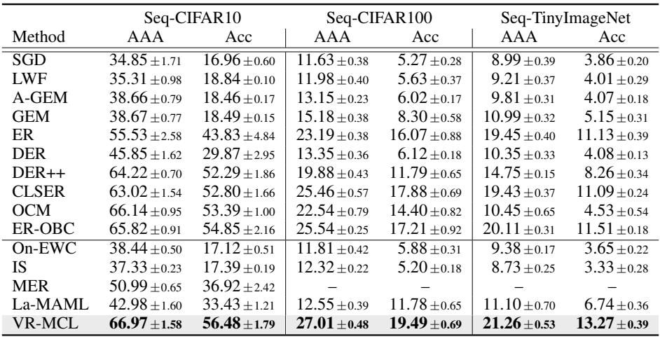
Experiments on Seq-CIFAR10, Seq-CIFAR100, and Seq-TinyImageNet under online continual learning evaluate VR-MCL against representative regularization, meta-learning, and state-of-the-art baselines using averaged and anytime accuracy. The results show that VR-MCL consistently improves performance across benchmarks, smaller memory buffers, diverse backbone architectures, and increasingly imbalanced nonstationary settings, while also outperforming alternative variance-reduction strategies. Ablation studies further confirm that the method effectively reduces gradient variance and better exploits second-order information, supporting its robustness and practical effectiveness.

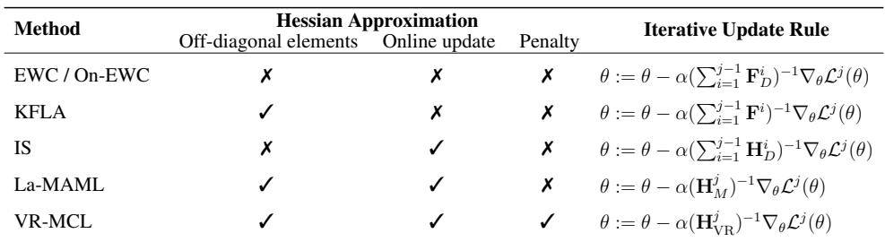
The table compares continual learning methods by expressing them as iterative updates that differ in how accurately and adaptively they approximate Hessian curvature. Simpler regularization methods use static diagonal Fisher estimates, while more advanced variants incorporate full Fisher information, online Hessian estimates, and eventually a regularized online Hessian. The regularized online Hessian used by VR-MCL is designed to reduce variance and improve stability under online continual learning. EWC and On-EWC use a limited diagonal Fisher approximation in the unified update rule. KFLA extends the comparison by including off-diagonal Fisher information. Importance sampling and La-MAML use online updates, with La-MAML also capturing off-diagonal structure. VR-MCL combines online Hessian estimation, off-diagonal structure, and a penalty term to obtain a more stable update. The paper reports that the regularized Hessian approximation helps under online continual learning, imbalanced task streams, and a smaller backbone network.

On reduced ResNet-18 with a small memory buffer, replay and gradient-constrained methods outperform plain SGD on Seq-CIFAR10, Seq-CIFAR100, and Seq-TinyImageNet. Experience replay yields the largest gains, while all methods struggle more as task sequences become longer and datasets become more complex. Final accuracy is consistently lower than averaged anytime accuracy, showing that performance degrades during streaming training. Experience replay is the most competitive baseline across all three online continual learning benchmarks GEM improves over plain SGD and becomes relatively more helpful on longer task sequences DER remains much weaker than experience replay, making replay alone the stronger approach among the listed methods Accuracy falls sharply when moving from Seq-CIFAR10 to Seq-CIFAR100 and Seq-TinyImageNet

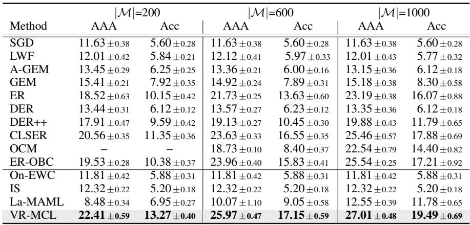
The table reports averaged final and anytime accuracy with 95% confidence intervals on Seq-CIFAR100 using reduced ResNet-18, and unstable results are omitted. Across buffer sizes, ER is the only method shown with a clear increase in both metrics as the buffer grows, while several other baselines remain flat or fluctuate. This suggests that larger memory helps most when the method can effectively exploit replayed examples. ER improves consistently from smaller to larger memory buffers in both averaged anytime and final accuracy. SGD, LWF, A-GEM, GEM, and DER show little consistent benefit from increasing memory size.

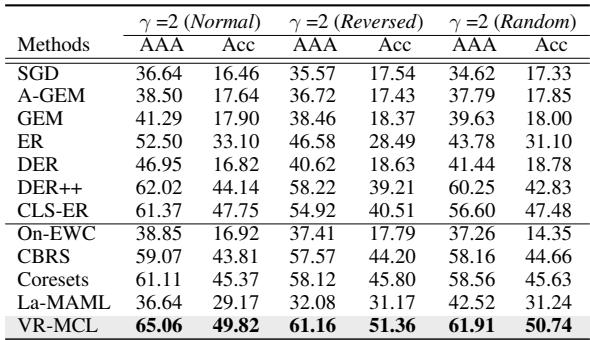
In the imbalanced Seq-CIFAR10 setting with ratio 2, replay-based methods generally perform better than basic SGD and gradient-projection baselines across normal, reversed, and random ordering. Final accuracy is consistently lower than averaged anytime accuracy for most methods, showing that later imbalance can degrade retention of earlier tasks. The surrounding analysis reports that VR-MCL remains the strongest method under this imbalanced setting, even compared with approaches designed for imbalanced continual learning. Replay-style baselines such as ER and DER++ show clearer gains over regularization-based and naive baselines in the visible results. Normal ordering usually gives higher averaged accuracy than reversed and random ordering for most baselines.

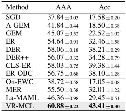
On Seq-CIFAR10 using the small PcCNN network with 200 memory samples, replay-based baselines outperform plain SGD and regularization-only approaches. The paper reports that VR-MCL improves by nearly 3 percent over the best baseline on both averaged any-time accuracy and final accuracy. These comparisons are based on 5-run averages with 95 percent confidence intervals. Replay-based methods achieve stronger accuracy than plain SGD on the small backbone VR-MCL gives nearly 3 percent gains over the best baseline in both accuracy metrics CLS-ER and DER are among the strongest reported baselines

Experiments compare continual learning methods across online continual learning benchmarks and ablations on a small ResNet-18 and a compact PcCNN, evaluating replay, regularization, and gradient projection under standard and imbalanced task streams. These tests validate that replay generally stabilizes performance and benefits most from larger memory, while accuracy drops on longer or harder sequences and from anytime to final scores. VR-MCL is shown to provide more stable online updates and stronger performance, especially in imbalanced streams and smaller-backbone settings, than conventional baselines.