One-sentence Summary

A review by researchers from the German Aerospace Center, Technical University of Munich, University of Zurich, and others examines the recent advances and challenges of deep learning in remote sensing, urging remote sensing scientists to integrate their domain expertise into deep learning as an implicit general model to address large-scale challenges such as climate change and urbanization.

Key Contributions

• The paper surveys deep learning for remote sensing, highlighting that deep neural networks consistently outperform hand-crafted feature methods, with most research concentrated on classification and detection tasks using benchmark datasets.
• It identifies technical challenges including limited annotated data, global-scale transferability, and the need for weakly-supervised or unsupervised learning, and reviews approaches such as never-ending learning and self-taught learning.
• The work provides resources like the 2017 IEEE GRSS Data Fusion Contest dataset and the Functional Map of the World Challenge dataset, and advocates for fusing physics-based models with deep learning to address large-scale problems like climate change and urbanization.

Introduction

Deep learning has transformed computer vision, and its adoption in remote sensing is accelerating as satellite data volumes explode and computational resources grow. Remote sensing imagery presents unique challenges that prior deep learning approaches do not fully address: data are often multi-modal (optical and SAR), geo-located, acquired with varying sensor quality, and inherently temporal; they demand not only classification but also retrieval of geophysical quantities, and must be processed at global scale. The authors review the current state of the art in deep learning for remote sensing, covering hyperspectral imaging, SAR, very high resolution analysis, data fusion, and 3D reconstruction, while also providing practical tools and open resources for the community.

Dataset

The authors present a curated list of open remote sensing datasets suitable for training deep neural networks, grouped by task. The datasets are described as resources for developing and benchmarking models, and the paper outlines their composition, sources, and typical usage.

Scene classification datasets (single label per image)

• UC Merced dataset – 2,100 RGB images (256×256 pixels) of 21 land use classes, 100 images per class. Used for whole-image classification. Source: UC Merced Vision Lab.
• AID dataset – 10,000 annotated aerial images across 30 scene classes. Larger and more diverse than UC Merced, aligning with modern deep learning data needs. Source: Wuhan University.
• NWPU-RESISC45 dataset – 31,500 images over 45 scene classes, the largest land use scene classification dataset in both total images and class count. Source: Northwestern Polytechnical University.

Image classification datasets (pixel-wise semantic labeling)

• Zurich Summer Dataset – 20 image chips from a QuickBird scene over Zurich, pansharpened to 0.6 m resolution, with 8 land use classes and ground truth labels. Source: Michele Volpi’s research site.
• Zeebruges (Data Fusion Contest 2015) – 7 tiles of 10,000×10,000 pixels, each with a 5 cm resolution RGB image and a dense LiDAR point cloud (65 pts/m²). Densely labeled into 8 land/object classes. Five tiles are provided with labels for training; the remaining two are used for evaluation via upload to the DASE server.
• ISPRS 2D Semantic Labeling Challenge – Sub-decimeter imagery over Vaihingen and Potsdam. Vaihingen: 33 tiles (~2000×3000 pixels), half labeled, half unlabeled for evaluation. Potsdam: 24 labeled tiles (6000×6000 pixels) and 14 unlabeled for evaluation. Height data (digital surface model) and an infrared channel are included. Labels cover 6 classes plus a clutter class. Evaluation uses withheld unlabeled tiles.

Registration/matching dataset

• SARptical Dataset – 10,000 pairs of precisely co-registered SAR and optical image patches from central Berlin. Built from 3D InSAR point clouds (TerraSAR-X) and 3D optical point clouds (UltraCam, 20 cm ground spacing). Intended for training and testing SAR-optical coregistration and matching algorithms. Source: Technical University of Munich.

The paper highlights these datasets as off-the-shelf benchmarks for training deep learning models. The datasets come with predefined splits where applicable: Zeebruges and ISPRS provide fixed training and evaluation tiles; SARptical offers paired patches for registration tasks; scene classification datasets are typically partitioned randomly for training and testing. No additional cropping or metadata construction is performed by the authors; the datasets are used as released, after standard preprocessing such as pansharpening or LiDAR rasterization.

Method

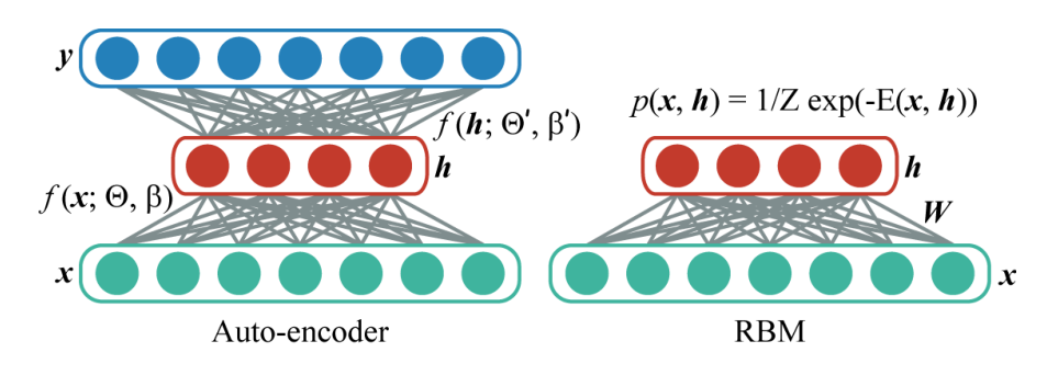
The authors leverage autoencoder models as a fundamental class of deep learning architectures for feature representation. A standard autoencoder maps an input $\pmb{x} \in \mathbb{R}^D$x∈RD to a latent representation $\pmb{h} \in \mathbb{R}^M$h∈RM via a nonlinear mapping $\boldsymbol{h} = f(\boldsymbol{\Theta}\boldsymbol{x} + \boldsymbol{\beta})$h=f(Θx+β). The encoded feature is then used to reconstruct the input $\pmb{y} = f(\boldsymbol{\Theta}'\boldsymbol{h} + \boldsymbol{\beta}')$y=f(Θ′h+β′). The parameters are optimized by stochastic gradient descent (SGD) to minimize the Euclidean distance between $\pmb{x}$x and $\pmb{y}$y. Stacked Autoencoders (SAE) consist of multiple layers where outputs of one layer feed into the next. To handle cases where the latent dimension exceeds the input dimension ($M > D$M>D), Sparse Autoencoders enforce a sparsity constraint on hidden units by minimizing a loss function that includes a Kullback-Leibler (KL) divergence penalty term. Unlike deterministic autoencoders, Restricted Boltzmann Machines (RBM) are stochastic undirected graphical models with visible and hidden layers. The energy function is defined as $\mathbb{E}(\boldsymbol{x}, \boldsymbol{h}) = \frac{1}{2}\boldsymbol{x}^T\boldsymbol{x} - (\boldsymbol{h}^T\boldsymbol{W}\boldsymbol{x} + \boldsymbol{c}^T\boldsymbol{x} + \boldsymbol{b}^T\boldsymbol{h})$E(x,h)=21​xTx−(hTWx+cTx+bTh). Stacking RBMs forms a Deep Belief Network (DBN), which is trained via a greedy layer-wise approach.

Refer to the framework diagram:

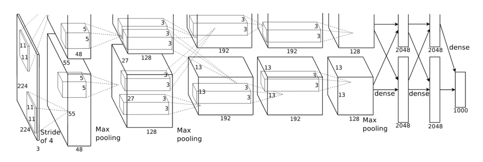
The authors review successful Convolutional Neural Network (CNN) architectures that have advanced computer vision. AlexNet scales earlier insights into a deeper network, utilizing rectified linear units (ReLU) to decrease training time, dropout layers to avoid overfitting, and data augmentation techniques. It was notably trained on GPUs to handle larger datasets and images. VGG Nets emphasize simplicity and depth, strictly using $3 \times 3$3×3 filters and $2 \times 2$2×2 max-pooling layers, reinforcing the notion that deeper architectures promote hierarchical feature representations. ResNet addresses the degradation problem in very deep networks by adding shortcut connections that perform identity mapping, bypassing stacked convolutional layers to facilitate optimization. Fully Convolutional Networks (FCN) are pivotal for semantic segmentation, employing an encoder/decoder structure for end-to-end learning of upsampling and skip connections for multi-scale inference.

As shown in the figure below:

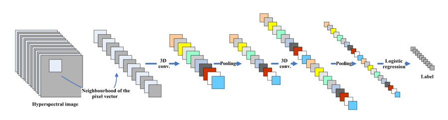
The authors apply deep learning to hyperspectral data analysis, particularly for classification tasks. Deep learning architectures extract high-level, hierarchical features that are robust to the nonlinear nature of hyperspectral imaging caused by atmospheric scattering and light mechanisms. Autoencoders, such as stacked autoencoders and DBMs, are used to extract hierarchical spectral features from unlabeled data. Supervised CNNs are employed in 1D, 2D, and 3D configurations. While 1D and 2D CNNs process spectral or spatial information respectively, 3D CNNs perform spatial-spectral convolution operations, modeling spectral information more effectively by treating the spectral dimension similarly to a time axis.

Refer to the framework diagram:

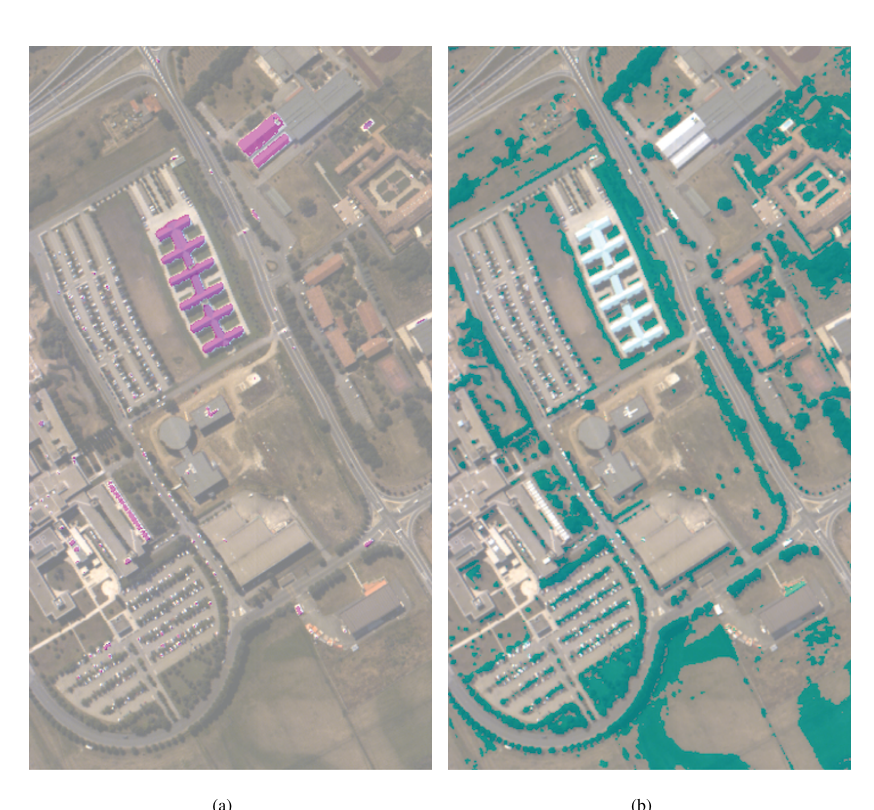
For unsupervised feature extraction, the authors discuss convolutional networks using sparse learning for greedy layer-wise weight estimation. A fully Residual Conv-Deconv network is proposed for unsupervised spectral-spatial feature learning. The learned filters in this network demonstrate significant description power for semantic visual patterns at the object level, effectively capturing features like metal sheets and vegetative covers.

As shown in the figure below:

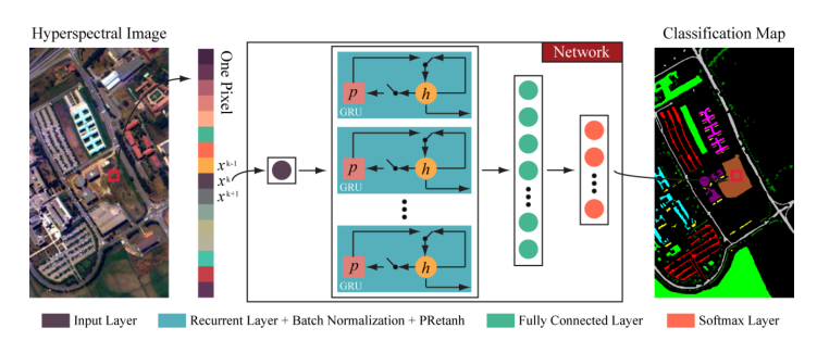
Additionally, Recurrent Neural Networks (RNN) are utilized for hyperspectral image classification. The authors propose an RNN model with a modified gated recurrent unit (GRU) and a new activation function. This architecture effectively analyzes hyperspectral pixels as sequential data, determining information categories via network reasoning.

Refer to the framework diagram:

Experiment

The reviewed experiments evaluate deep learning across hyperspectral image classification, SAR target recognition and terrain analysis, high-resolution satellite scene classification and object detection, and 3D reconstruction from imagery. Deep architectures, especially CNNs, consistently outperform traditional hand-crafted feature methods by learning hierarchical and discriminative representations, yet they often suffer from overfitting due to limited labeled remote sensing data, leading to reliance on data augmentation, transfer learning, or smaller network designs. The integration of deep learning has also enabled qualitatively new outcomes such as semantically labeled 3D models and fully learned stereo pipelines. Overall, deep learning significantly advances remote sensing interpretation, but data scarcity remains a central practical challenge.

CNN-based stereo methods dominate the ranking, achieving substantially lower bad pixel error rates than the traditional SGM method. The top entry, 3DMST, attains a 5.92% error rate, while SGM records 18.4%, highlighting the impact of learned features on depth estimation accuracy. CNN-based methods occupy the four leading positions, with error rates ranging from 5.92% to 8.08%. The classic SGM approach trails significantly, with an error rate more than double that of the best CNN-based method.

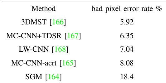
The evaluation compares stereo depth estimation methods on a standard benchmark, contrasting traditional SGM against several CNN-based approaches. The results clearly show that learned features provide a decisive advantage, with CNN-based techniques occupying the top ranks and delivering substantially lower error rates. This demonstrates that deep learning significantly improves accuracy over classical hand-crafted methods.