One-sentence Summary

FAIR (Meta) and the Weizmann Institute of Science propose Riemannian Flow Matching (RFM), a simulation-free framework for continuous normalizing flows on manifolds that constructs a premetric enabling closed-form target vector fields and leverages spectral decompositions to extend to general geometries, achieving state-of-the-art results on non-Euclidean datasets including triangular meshes.

Key Contributions

• Riemannian Flow Matching (RFM) trains continuous normalizing flows on manifolds by regressing closed-form conditional vector fields rather than score functions, yielding simulation-free training on simple geometries and avoiding divergence computation during training.
• RFM introduces a premetric for defining target vector fields and uses spectral decompositions to approximate it efficiently on general geometries, enabling tractable training with approximate spectral distances under finite truncation.
• RFM achieves state-of-the-art performance on real-world non-Euclidean datasets and demonstrates tractable training on general geometries, including triangular meshes with non-trivial curvature and boundaries.

Introduction

The authors focus on generative modeling for data that live on Riemannian manifolds, such as spheres, hyperbolic spaces, product geometries, and meshes. This matters because many real-world datasets have geometric constraints, and Euclidean generative methods do not naturally respect these structures.

Prior manifold-aware continuous normalizing flow and diffusion models face important limitations. Some require simulation or iterative sampling during training, even on simple geometries. Others scale poorly to high dimensions, rely on approximations to score functions or divergences, or need difficult stochastic differential equation solvers on manifolds.

The authors leverage the Flow Matching framework to introduce Riemannian Flow Matching, a scalable method for learning continuous normalizing flows directly on general Riemannian manifolds. Their key idea is to regress a target vector field onto conditional vector fields built from a manifold premetric, naturally the geodesic distance. This yields a simple training objective, avoids divergence estimation, and becomes fully simulation-free on geometries with closed-form geodesics while remaining practical on more general manifolds.

Method

The authors leverage a Riemannian flow matching framework to train a generative model on a smooth manifold. The manifold is assumed to be complete, connected, and equipped with a metric $g$g. Training samples are drawn from an unknown data distribution $q(x_1)$q(x1​) on the manifold, while the model aims to transform a simple base distribution $p$p into $q$q. Rather than learning the final transport map directly, the method learns a time dependent tangent vector field

parameterized by $\theta$θ. This vector field defines a continuous normalizing flow on the manifold by solving an ordinary differential equation. The learned flow transports points from the base distribution toward the data distribution over time.

The core training objective is to fit the parametric vector field $v_t$vt​ to a known target vector field $u_t$ut​ that generates a desired probability path $p_t$pt​ on the manifold. The probability path must satisfy the boundary conditions

On a Euclidean domain, this resembles flow matching. On a manifold, tangent vectors are compared using the Riemannian metric, giving the objective

Here $v_t(x)$vt​(x) and $u_t(x)$ut​(x) both lie in the tangent space at $x$x, and the norm is induced by the manifold metric $g$g.

A direct target path $p_t$pt​ and velocity field $u_t$ut​ are generally intractable. The authors therefore construct conditional probability paths $p_t(x \mid x_1)$pt​(x∣x1​), where each condition is a training sample $x_1$x1​. Each conditional path starts from the base distribution and collapses onto the data point $x_1$x1​ at the final time:

The marginal path is then obtained by averaging over the data distribution:

The corresponding marginal vector field can also be written as a conditional average, but evaluating it directly is expensive. The key training simplification is to replace the marginal matching loss with a conditional matching loss:

This loss is equivalent to the original flow matching objective under the conditional construction, but it only requires sampling from a tractable conditional path.

The practical training pipeline samples a time $t$t, a data point $x_1$x1​, and a base point $x_0$x0​. The method then constructs a conditional flow

and uses the time derivative

as the regression target. The resulting training objective becomes

At each update, the model only needs to evaluate $v_t(x_t; \theta)$vt​(xt​;θ) and compare it with the target tangent vector. If the conditional flow does not have a closed form, $x_t$xt​ can be obtained by forward simulation of the conditional vector field. Gradients are taken with respect to the model parameters, while the simulation itself does not need to be differentiated through.

The central design module is the construction of the conditional flow. The authors introduce a premetric $d: \mathcal{M} \times \mathcal{M} \rightarrow \mathbb{R}$d:M×M→R to measure how close a point is to the conditioning point $x_1$x1​. The premetric is required to be nonnegative, positive only for identical points, and nondegenerate in the sense that its gradient is nonzero away from the conditioning point. These properties ensure that decreasing the premetric leads all points toward $x_1$x1​.

Given a scheduler $\kappa(t)$κ(t) satisfying

the desired conditional flow reduces the premetric according to

A conditional vector field that realizes this contraction is

The scheduler controls the speed of contraction. A particularly simple choice is linear decay,

which yields a conditional flow that reduces the premetric at a constant relative rate. With this scheduler, the training loss can be written as

When the premetric is chosen to be the geodesic distance $d_g$dg​, the resulting conditional flow becomes especially natural. In that case, the vector field is the minimal norm solution that decreases the distance to $x_1$x1​, and the corresponding trajectory is a constant speed geodesic connecting $x_0$x0​ to $x_1$x1​. On manifolds where geodesics have closed forms, the interpolated point can be written using the exponential and logarithm maps:

This makes the training objective simulation free for standard geometries such as Euclidean space, hyperspheres, hyperbolic spaces, tori, and certain matrix Lie groups. In Euclidean space, with the standard norm, the method recovers the familiar straight line interpolation and the corresponding Euclidean flow matching target.

For general manifolds, geodesics may be expensive to compute for arbitrary pairs of points. The authors therefore introduce spectral distances as efficient premetrics. These distances are constructed from the eigenfunctions and eigenvalues of the Laplace-Beltrami operator. If $\varphi_i$φi​ are eigenfunctions with eigenvalues $\lambda_i$λi​, a spectral distance has the form

where $w$w is a decreasing weighting function. Common choices include diffusion distance weighting,

and biharmonic distance weighting,

In practice, the infinite series is truncated to the smallest $k$k eigenvalues. The required eigenfunctions are computed once during preprocessing, after which the distance can be evaluated quickly during training. The authors note that a finite truncation is sufficient for the role of the premetric and does not introduce bias in the training procedure. For manifolds with boundaries, using Neumann boundary conditions when solving for eigenfunctions helps ensure that the induced conditional vector field remains inside the manifold. Unlike geodesic distance, spectral distances generally do not yield closed-form minimal paths, so the conditional flow must be obtained by simulation.

Experiment

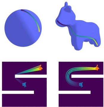
The experiments evaluate the method across spherical climate datasets, protein torsion-angle tori, high-dimensional tori, mesh manifolds, and maze-like manifolds with boundaries. Results show improved modeling of concentrated regions and complex distributions, with especially strong gains on higher-dimensional tori while avoiding approximation-induced instability in competing approaches. On curved mesh manifolds, spectral distances enable practical high-fidelity generation, and on bounded mazes the learned vector field successfully transports mass across non-trivial topology without crossing boundaries.

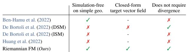
The comparison shows that Riemannian Flow Matching is the only listed method that combines simulation-free operation on simple geometries, a closed-form target vector field, and no need for divergence estimation. It also uniquely extends to general manifolds, while several related continuous-time or diffusion-inspired methods rely on simulation, score-function approximation, or variance-increasing divergence estimation. Riemannian Flow Matching remains simulation free on simple manifolds. It does not require divergence estimation. It is the compared approach that also handles general geometries.

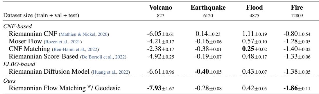
Across Earth and climate science datasets on the sphere, lower test negative log-likelihood shows different best methods by dataset. The strongest gains are reported for volcano and fire datasets, where concentrated regions make high-fidelity density modeling especially important. Volcano and fire results stand out as areas of notable improvement because their data concentrate in regions that require accurate density modeling. Among the listed methods, performance is split across the remaining sphere datasets, with ELBO-based Riemannian diffusion strongest on Earthquake and CNF matching strongest on Flood.

The protein dataset results show that Riemannian Flow Matching with a geodesic construction improves test negative log-likelihood on most 2D and 7D torus datasets compared with prior Mixture of Power Spherical and Riemannian Diffusion baselines. The advantage is especially clear on the higher-dimensional RNA dataset, while the diffusion baseline remains slightly stronger on one 2D dataset. This supports the method's scalability for more complex torsion-angle distributions. Riemannian Flow Matching with a geodesic construction achieves the best or near-best performance across most protein torus datasets. The method shows a particularly strong relative gain on the higher-dimensional RNA dataset. Prior Riemannian Diffusion still obtains the best result on the Proline 2D dataset.

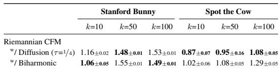
On mesh manifolds, model performance varies with the chosen spectral distance and the number of eigenfunctions used. The biharmonic distance is described as smoother and easier to use, and it often yields lower test negative log-likelihood on the Stanford Bunny mesh, while the diffusion distance performs better on the Spot the Cow mesh. Across both distance choices, test error tends to rise as more eigenfunctions are used. Biharmonic distance can outperform diffusion distance on the Stanford Bunny mesh at several eigenfunction counts. Diffusion distance gives lower test negative log-likelihood than biharmonic distance on the Spot the Cow mesh across the reported settings.

The experiments evaluate the proposed method across theoretical properties and practical density estimation tasks on sphere, torus, and mesh manifolds. The comparison highlights that Riemannian Flow Matching uniquely combines simulation-free operation, a closed-form target vector field, no divergence estimation, and applicability to general geometries, while empirical results on Earth and climate datasets show dataset-dependent advantages, with especially strong gains for highly concentrated volcano and fire data. Further evaluations on protein torus manifolds demonstrate strong density estimation performance and scalability, particularly for higher-dimensional structures, whereas mesh experiments show that outcomes depend on the chosen spectral distance and scale, indicating robustness across varied manifold geometries.