One-sentence Summary

LSD-SLAM, proposed by researchers at Technical University Munich, is a direct monocular SLAM system that operates on $sim(3)$sim(3) to explicitly detect scale drift and employs a probabilistic formulation to incorporate noisy depth values into tracking, enabling large-scale, consistent mapping with real-time semi-dense depth reconstruction on a CPU.

Key Contributions

• LSD-SLAM is introduced as a direct, featureless monocular SLAM algorithm that combines accurate pose estimation from direct image alignment with large-scale, consistent environment reconstruction. It maintains a pose graph of keyframes with probabilistic semi-dense depth maps obtained from many pixelwise small-baseline stereo comparisons.

• A novel direct tracking method aligns keyframes using Sim(3) similarity transformations, explicitly modeling and detecting scale drift in monocular trajectories. This scale-aware formulation enables reliable tracking and mapping across sequences with large scene-scale variations.

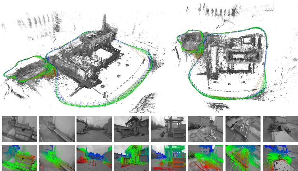
• The method incorporates a probabilistic treatment of depth-map uncertainty into direct tracking to account for noisy depth estimates. Experiments show that the resulting CPU-real-time system tracks and maps hand-held trajectories over more than 500 m, including large rotations and scale variations with average inverse depth from less than 20 cm to more than 10 m.

Introduction

Monocular SLAM and 3D reconstruction matter for UAV navigation, augmented reality, and virtual reality because a single camera can operate across many environment scales without depth or stereo range limits. The main challenge is scale ambiguity, since a monocular camera cannot directly measure absolute world scale and scale drift becomes a major source of error. Feature-based methods are limited because they only use feature observations, discarding useful edge and region structure, while prior direct monocular methods used full image intensities but only produced local odometry without a consistent global map. The authors leverage direct image alignment and semi-dense depth estimation to present LSD-SLAM, a direct monocular SLAM framework that builds a global pose graph of keyframes. Its key contribution is using similarity transforms to explicitly model scale drift, along with probabilistically incorporating depth uncertainty into tracking, enabling real time performance on a CPU and more robust large-scale mapping.

Method

The authors leverage a direct monocular SLAM pipeline that operates continuously on image streams and represents the environment as a pose graph of keyframes. Refer to the framework diagram:

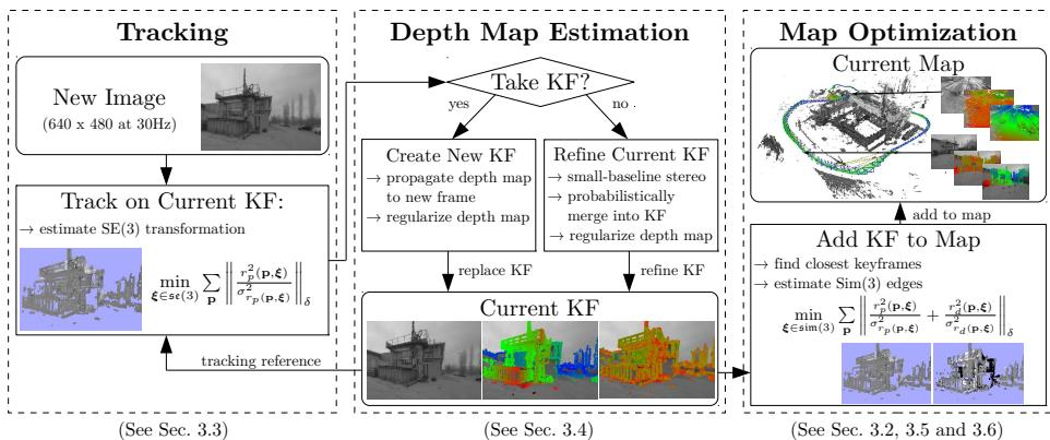
The framework consists of three tightly coupled modules: tracking, depth map estimation, and map optimization. The tracking module estimates the relative pose of new images with respect to the current reference keyframe. The depth map estimation module either refines the current keyframe or creates a new one when the camera moves sufficiently far. The map optimization module incorporates replaced keyframes into a global pose graph, where relative transformations and uncertainties are refined to reduce accumulated drift.

Each keyframe contains an intensity image, an inverse depth map, and the variance of that inverse depth map. The depth values and variances are semi dense, meaning they are maintained only in image regions with sufficient intensity gradient. Edges in the map store similarity transformations between keyframes together with associated covariance matrices. The first keyframe can be initialized with random inverse depth values and large variance. With sufficient translational motion, the system converges toward a stable depth configuration without requiring a separate dense initialization procedure.

At the lowest level, image alignment is performed by minimizing a photometric error. Given a reference keyframe $\kappa_i$κi​ with image $I_i$Ii​, inverse depth map $D_i$Di​, and depth variance $V_i$Vi​, a new image $I_j$Ij​ is aligned by estimating a relative transformation $\boldsymbol{\xi}_{ji}\in\mathfrak{se}(3)$ξji​∈se(3). The residual for a pixel $\mathbf{p}$p is

The optimization objective is a variance normalized robust photometric error:

The Huber style robust norm is defined as

The key design choice is that the residual variance is not assumed constant. The authors compute

where $\sigma_I^2$σI2​ models image intensity noise and $V_i(\mathbf{p})$Vi​(p) models uncertainty in the inverse depth map. As shown in the figure below:

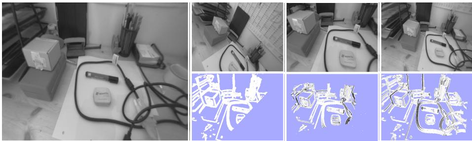
The figure illustrates how the normalization changes with motion type. For pure rotation, depth uncertainty does not affect photometric residuals, so the normalization remains uniform. For forward motion, the effect is concentrated in specific image regions. For lateral motion, residuals are weighted differently depending on the local intensity gradient direction. This behavior is important because monocular depth uncertainty is highly spatially variable.

The alignment itself is solved by an iteratively reweighted Gauss Newton optimization on a Lie group. The residual vector is $\mathbf{r}=(r_1,\ldots,r_n)^T$r=(r1​,…,rn​)T, and a left compositional update is used. In each iteration, the update is computed as

followed by

The weight matrix $\mathbf{W}$W downweights pixels with large residuals, making the estimator robust to occlusions, reflections, and other photometric violations. The inverse weighted Hessian estimate

is used to describe the uncertainty of the final pose. The authors use a left multiplication convention, meaning the final pose can be expressed as

Residuals are generally correlated in practice, so this covariance is treated as a lower bound rather than a fully exact model. Nevertheless, it provides useful information for robust matching, loop closure checking, and global pose graph optimization.

Uncertainty is propagated through nonlinear functions using a Jacobian based approximation. If an input variable $\mathbf{X}$X has covariance $\boldsymbol{\Sigma}_{\mathbf{X}}$ΣX​, and the output is $\mathbf{Y}=f(\mathbf{X})$Y=f(X), then the output covariance is approximated by

This mechanism allows the depth variance $V_i$Vi​ to be incorporated into the photometric residual variance used during tracking.

The depth map estimation module decides whether to refine the current keyframe or promote the latest tracked frame into a new keyframe. The keyframe selection criterion uses a weighted distance measure

where $\mathbf{W}$W balances relative translation and rotation. If the threshold is exceeded, the system creates a new keyframe by projecting depth from existing nearby keyframes into the new image. One iteration of spatial regularization and outlier removal is then applied. The new depth map is scaled so that its mean inverse depth equals one, and the corresponding scale is absorbed into the keyframe’s similarity transformation pose.

If the new frame does not become a keyframe, it is used to refine the current keyframe. The authors employ many efficient small baseline stereo comparisons in regions with high expected stereo accuracy. The resulting measurements are probabilistically merged into the existing inverse depth map, while regularization maintains spatial consistency.

For global consistency, the system performs direct image alignment on $\mathfrak{sim}(3)$sim(3) rather than only $\mathfrak{se}(3)$se(3). Monocular tracking is scale ambiguous, and this ambiguity causes scale drift over long trajectories. To address this issue, the authors normalize each keyframe so that its mean inverse depth is one and estimate inter keyframe constraints as similarity transformations. The optimization objective combines photometric and depth residuals:

The photometric residual has the same form as during tracking. The depth residual is

where

is the transformed point under the similarity transform. The depth residual variance is propagated from both keyframes:

The combined robust residual reflects the fact that photometric outliers and depth outliers often occur together. The depth term is required because photometric alignment alone cannot determine scale on $\mathfrak{sim}(3)$sim(3).

Candidate loop closure or large offset keyframe constraints are collected from nearby keyframes and from an appearance based mapping mechanism. Before inserting a constraint into the global graph, the authors perform a reciprocal tracking check. For a candidate pair, the system estimates both $\boldsymbol{\xi}_{j_k i}$ξjk​i​ and $\boldsymbol{\xi}_{i j_k}$ξijk​​. The two estimates are accepted only if their mismatch is statistically small:

The adjoint transformation maps the second covariance into the tangent space consistent with the first estimate. This reciprocal check helps suppress false loop closures.

Direct image alignment on $\mathfrak{sim}(3)$sim(3) is nonconvex and requires initialization. The system uses second order minimization techniques and a coarse to fine pyramid that starts at very low resolution, increasing the convergence radius for loop closure alignment. These choices help the method recover from larger initial errors than dense direct alignment normally allows.

The map optimization module continuously refines the pose graph in the background. The optimized variables are the absolute poses $\boldsymbol{\xi}_{W1},\ldots,\boldsymbol{\xi}_{Wn}$ξW1​,…,ξWn​ of keyframes with respect to the world frame. The objective is a Mahalanobis sum over relative similarity constraints:

This formulation follows the left multiplication convention used for local tracking. The resulting pose graph correction enforces global consistency by combining odometry constraints, loop closure constraints, and their estimated uncertainties.

Experiment

LSD-SLAM was evaluated both qualitatively on long, challenging outdoor trajectories and quantitatively on a public RGB-D benchmark adapted to monocular operation. The qualitative tests showed that the method can handle extensive rotations, large scale changes, complex depth variations, and major loop closures. The quantitative evaluation demonstrated competitive tracking accuracy on a difficult benchmark, while additional experiments showed that the proposed tracking steps substantially increase the convergence radius for sim(3) camera motion without noticeably reducing precision.

Across the TUM RGB-D and simulated sequences, LSD-SLAM generally produces lower absolute trajectory error than the monocular baselines, including a case where one baseline fails to track. It is also competitive with methods that use sensor depth, although a direct RGB-D approach has lower error on some TUM and slow-motion simulated sequences. LSD-SLAM outperforms semi-dense monocular odometry and keypoint-based monocular SLAM on the reported sequences, with the latter failing on one TUM sequence. LSD-SLAM remains close to depth-based RGB-D SLAM despite using depth only for initialization, with depth methods leading on some sequences and LSD-SLAM leading on a simulated sequence.

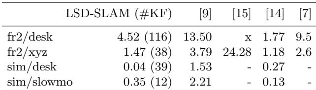
The experiments evaluate LSD-SLAM on TUM RGB-D and simulated sequences against monocular and depth-based baselines, primarily assessing absolute trajectory accuracy and tracking robustness. LSD-SLAM generally outperforms monocular methods, including semi-dense odometry and keypoint-based SLAM, which are less reliable on some sequences. It also remains competitive with depth-based RGB-D SLAM despite using depth only for initialization, showing that the proposed approach achieves strong overall performance across diverse sequence conditions.