Command Palette
Search for a command to run...
Scaling Harness Intelligence via Just-in-Time Harness Evolution
Scaling Harness Intelligence via Just-in-Time Harness Evolution
Abstract
Agent capability is not determined by the model alone. The agent harness, encompassing memory management, planning strategy, action protocol, and tool/skill orchestration, can dominate the contribution of the underlying foundation model. Yet harness design remains manual, task-specific, and fundamentally unscalable. We present JIT-Agent, a harness intelligence model trained to synthesize task-adaptive agent harnesses on the fly for arbitrary of-the-shelf agentic LLMs. We formalize the agent harness as a composable, machine-generatable artifact governed by a fixed four-module protocol, and train JIT-Agent to customize harnesses for a given task at hand, repair harnesses for stable and reliable execution, and self-evolve by distilling performance signals from an expanding archive of prior harness configurations. Equipped with JIT-Agent as a harness helper, DeepSeek-V4-Flash surpasses GPT-5.6 on DeepSearchQA (+9.1) and OdysseyBench (+4.3), while the already strong GLM-5.2 gains up to +20.2 points. Across controlled evaluations, JIT-Agentgenerated harnesses are performance-competitive with mature agent runtimes such as OpenCode and Claude Code and consistently improve multi-scale model families of DeepSeek V4, Mimo-V 2.5, and Qwen3.6. To our knowledge, JIT-Agent is the first model purpose-built for just-in-time harness generation, establishing harness intelligence as a trainable, transferable, and compounding dimension of agent capability orthogonal to model scaling.
One-sentence Summary
Researchers from Shanghai Jiao Tong University and collaborating institutions introduce JIT-Agent, the first harness intelligence model that synthesizes task-adaptive agent harnesses on the fly via a fixed four-module protocol, enabling repair and self-evolution; when paired with DeepSeek-V4-Flash, it surpasses GPT-5.6 on DeepSearchQA (+9.1) and OdysseyBench (+4.3), improves GLM-5.2 by up to +20.2 points, and matches mature runtimes like OpenCode and Claude Code.
Key Contributions
- Introduces JIT-Agent, a harness intelligence model that synthesizes task-adaptive agent harnesses at inference time for arbitrary off-the-shelf agentic LLMs, formalizing the harness as a composable artifact governed by a fixed four-module protocol (memory, planning, action, and tool/skill orchestration).
- Trains JIT-Agent through customization learning, repair supervision, and Evo-GDPO, enabling task-conditioned harness generation, repair from execution feedback, and self-evolution via distillation of performance signals from prior harness configurations, shifting harness construction from manual, ahead-of-time engineering to learned just-in-time optimization.
- Demonstrates that JIT-Agent-generated harnesses improve DeepSeek-V4-Flash by +9.1 on DeepSearchQA and +4.3 on OdysseyBench, surpassing GPT-5.6, and boost GLM-5.2 by up to +20.2 points, while remaining competitive with mature runtimes like OpenCode and Claude Code across multi-scale model families including DeepSeek V4, Mimo-V 2.5, and Qwen3.6.
Introduction
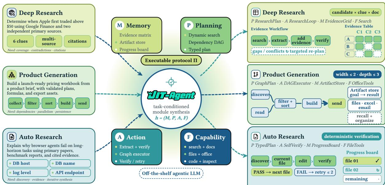
The authors address a key limitation in LLM agent design: agent capability depends not only on the foundation model but also on the harness that manages memory, planning, actions, and tool use. Prior work typically optimizes harnesses ahead of time (AOT), treating them as durable artifacts meant to generalize across tasks, which fails when deployment distributions are heterogeneous or instance-specific. To overcome this, the authors propose JIT-Agent, a compact meta-agent that generates task-specific harnesses just in time (JIT) at inference, wrapping an off-the-shelf agentic LLM for execution. The system is trained via a three-stage pipeline that teaches task-conditioned customization, repair from failed generations, and evolution through a novel optimization method called Evo-GDPO, shifting harness engineering from static artifacts to learned, on-the-fly synthesis.
Method
3 Unified Harness Codebase
3.1 Modularized Harness Design Space
An agent harness is the operational layer that turns a foundation model into a closed-loop agent: it determines what from prior interaction is retained, how intermediate directives are formed, which external capabilities are exposed at each stage, and how control advances. Harness generation is therefore defined over programs rather than unconstrained text. The authors distinguish the raw generation space G, syntactically valid harnesses Hsyn, protocol-compliant harnesses HΠ, and their executable subset HΠexec, with G⊇Hsyn⊇HΠ⊇HΠexec. The fixed protocol specifies module schemas and interfaces, their lifecycle, validation rules, and the shared execution semantics. It removes incidental variation in language and runtime while retaining the principal operational choices that distinguish existing harnesses.
Harness Composability. Composability has become a first-class concern in modern harness design. DeepSeek Harness, for example, adopts an "Everything is a Plugin" architecture, representing the runtime as modules connected through explicit dependency relationships. Composability is equally central to just-in-time (JIT) generation: it turns harness construction from unconstrained program synthesis into assembly over a typed, recombinable design space.
JIT-Agent makes these choices explicit through four interoperable modules: how history is compressed, how local intent is formed, how tools and skills are orchestrated, and how control advances. Let τ be a task, πψ a frozen backbone executor, and Cτ the capability registry available (e.g., tools, APIs, skills) to that task. Running a harness h with πψ induces a closed-loop trajectory
ξ∼Rollout(τ,πψ,h,Cτ;Π)=(s1,e1,o1,…,sT,eT,oT),where st∈S is the maintained controller state, et is the emitted tool call or terminal output, ot∈O is the resulting observation, and T is the protocol- or budget-bounded stopping time. The key assumption is that every h∈HΠ admits the modular factorization
h=(M,P,A,F)∈M×P×A×F,where M, P, A, and F denote memory, planning, action, and capability-orchestration modules, and M, P, A, and F are their protocol-compatible implementation spaces. The tuple follows this conceptual decomposition; at runtime, its dependency order is M→P→F→A. All modules operate against the same frozen backbone, whose common runtime dependence is suppressed below.
Position. Production harnesses such as Codex, Claude Code, and DeepSeek Harness expose substantially richer mechanisms than the four-module instantiation. That gap is deliberate. This work does not ask a model to reproduce an entire production runtime, but rather establishes a more fundamental result: even compact harnesses, generated just in time, can yield substantial gains. The JIT paradigm is complementary to production harness engineering. As models increasingly participate in the design and revision of their own runtimes, the training recipe for harness intelligence will matter at larger scales as well. The authors view the present design space as a starting point.
The protocol maintains both the immutable event history ξ<t and the mutable controller state st, which interact as
vt=M(ξ<t,st)∈V,history→view, dt=P(τ,st,vt)∈Ddir,view→local directive, Ct=F(Cτ,st,vt,dt)⊆Cτ,directive-conditioned capability orchestration, (st+1,et)=A(st,τ,vt,dt,Ct)∈S×A,control update and action emission,where V and Ddir are the view and directive spaces, and A=U⊔Y is the disjoint union of executable calls and terminal outputs. The registry Cτ contains callable tools (e.g., bash tools, APIs, and MCPs) as well as higher-level agent skills. A harness without an explicit planner remains type-consistent through the null directive d∅∈Ddir, returned by P∅ at every step. That is, memory constructs a view of realized history, planning converts that view into a local directive, capability orchestration activates the relevant external tools or agent skills, and the action module consumes the assembled context to both update the controller state and emit the next action. The kernel then interprets the emitted action by
ot={Exec(et;Ct),⊥,et∈U,et∈Y,ξ≤t=ξ<t⊕(st,et,ot),where Exec:U×2Cτ→O is the shared execution kernel, ⊥∈O is the terminal null observation, and ⊕ appends an event to the trajectory. Execution starts from ξ<1=∅ and a protocol-defined initial state s1∈Sinit, and terminates when et∈Y, yielding y=eT∈Y. This factorization turns otherwise heterogeneous programs into comparable coordinates in M×P×A×F.
Canonical ReAct can be written as hReAct=(Mfull,P∅,Areact,Fall), where Areact is the standard ReAct loop, P∅ denotes the absence of an explicit planner, Mfull keeps the running history without context management, and Fall exposes the full tool/skill registry. Engineered ReAct variants like Codex and OpenCode still fit the same scaffold: (Mcompact,Ptodo,Areact,Fall), where the action kernel remains ReAct-style, but Mcompact compresses history near the context limit and Ptodo maintains an explicit task todo list. Recursive architectures such as ROMA, AOrchestra, and Recursive Language Models (RLM) are likewise captured by choices such as hrec=(Msubproblem,Pdecomp,Arec,Froute). In such systems, the main orchestrator may spawn subagents through Arec, maintain a todo-style decomposition in Pdecomp, keep agent contexts isolated in Msubproblem, and allocate tools or skills to each subagent through Froute.
Given this modularized design space, the authors next introduce HarnessFactory, whose role is to test the expressiveness of HΠ and furnish diverse source material for JIT-Agent's meta-harness design.
3.2 HarnessFactory
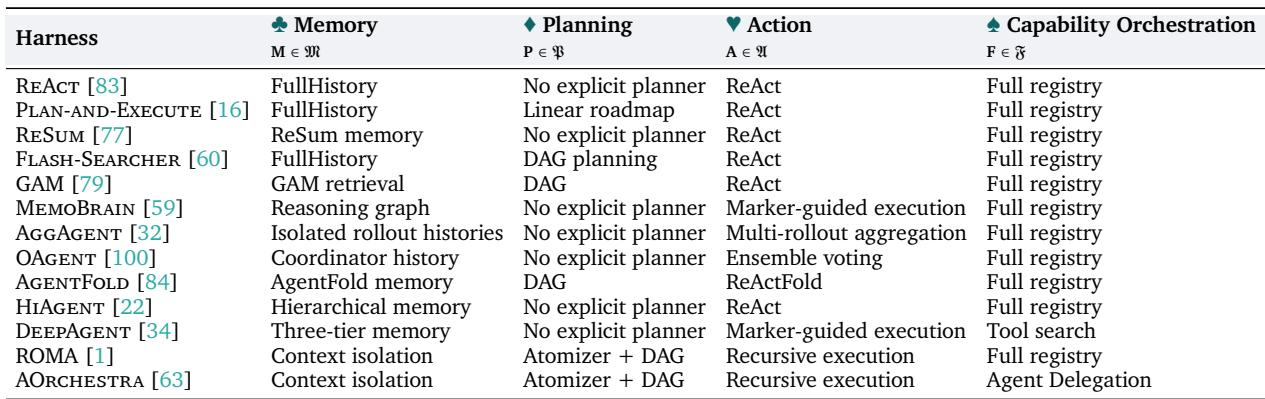
Under the shared protocol and a common kernel, HarnessFactory re-implements 13 representative contemporary agentic scaffolds: ReAct, Plan-and-Execute, ReSum, Flash-Searcher, General Agentic Memory (GAM), MemoBrain, AggAgent, OAgent, AgentFold, HiAgent, DeepAgent, ROMA, and AOrchestra. They provide heterogeneous memory, planning, action, and capability-orchestration strategies. The seed bank B0 therefore contains K0=13 protocol-compatible harnesses.
The bank serves a dual role: harnesses sampled from B0 anchor Stage-I synthesis, while later archive states supply the prior population against which new designs are evaluated. As the system operates, B0 grows into Bn⊇B0, whose entries associate each retained harness with its task and observed reward, latency, and cost; this evolution is formalized in Section 4.3.
4 Training Pipeline
Training follows the inference-time lifecycle of JIT-Agent: first synthesize a task-conditioned harness, then recover unstable generations, and finally learn to improve from stronger archive states online. Let τ∼Dtask denote a task drawn from the training distribution, Cτ its capability registry, and Eτ a small reference context from the harness bank. The authors define the generation context as cτ=(τ,Π,Cτ,Eτ) and sample harnesses from pθ(h∣cτ). A frozen executor πψ∼M then runs each harness for validation and utility measurement. The common objective is
θ⋆=argθmaxEτ∼Dtask,πψ∼M,h∼pθ(⋅∣cτ)[U(τ,πψ,h)],where U evaluates the trajectory induced by the model-harness pair using task reward, latency, and monetary cost. Because pθ generates in G rather than satisfying executability by construction, every output is checked by the protocol validator. The authors use ValidΠ(h;τ,πψ,Cτ)∈{0,1} for its validity flag; failed checks additionally return a structured diagnostic report. They instantiate Equation (8) with offline supervision in Stage I, repair-trajectory learning in Stage II, and online policy improvement in Stage III.
4.1 Stage I: Customizing Harness
Data Preparation. Stage I uses a frozen, stronger teacher qϕ to synthesize task-adapted harnesses under the fixed four-module protocol. For each task, three reference scaffolds are sampled from the task-type-matched subset B0(d(τ)) of the seed bank,
Eτ={h(1),h(2),h(3)}∼Sample3(B0(d(τ))),hteach∼qϕ(⋅∣cτ),where d(τ) denotes the task type. The teacher receives the task, protocol, capability registry, and sampled scaffolds. A generation is retained only if it passes protocol validation and execution checks, yielding
DI={(τ,πψ,Cτ,Eτ,hteach)∣ValidΠ(hteach;τ,πψ,Cτ)=1}.Stage I draws its training tasks from different sources, including existing benchmarks as well as a portion of synthesized tasks.
Training Setup. Stage I uses two coupled objectives. The first is a standard supervised fine-tuning objective over accepted teacher generations:
LIgen(θ)=−E(τ,πψ,Cτ,Eτ,hteach)∼DIj=1∑∣hteach∣logpθ(yjteach∣y<jteach,cτ),where yjteach is the j-th target token. This teaches JIT-Agent to map a task and a small reference context directly to a protocol-compliant harness. Protocol compliance alone is insufficient: executable harnesses can still differ substantially in task reward, latency, and monetary cost. The authors therefore compare candidates under the same backbone and evaluation seeds, retaining a preference only when reward improves without degrading either efficiency axis and at least one efficiency gain is strict:
h+≻τh−⟺r+>r−∧ℓ+≤ℓ−∧κ+≤κ−∧(ℓ+<ℓ−∨κ+<κ−),Δval(τ;h+,h−)=αr(r+−r−)+αℓ[ℓ−−ℓ+]++ακ[κ−−κ+]+,where (r±,ℓ±,κ±) are repeated-rollout averages for (h+,h−), [x]+=max(x,0), and αr,αℓ,ακ≥0 control the three value gaps. Let DIpref collect the resulting preference tuples. The authors optimize the reference-anchored objective
LIpref(θ)=−E(τ,πψ,Cτ,Eτ,h+,h−)∼DIpref[Δval⋅logσ(βpreflogpθ(h−∣cτ)pθ(h+∣cτ)−βpreflogpref(h−∣cτ)pref(h+∣cτ))].Here σ is the logistic sigmoid, βpref>0 controls preference sharpness, and pref is the frozen Stage-I SFT checkpoint; in the log ratios, logp(h∣⋅) denotes length-normalized sequence log-likelihood. The full Stage-I objective is LI(θ)=LIgen(θ)+λprefLIpref(θ) with λpref≥0. Generation imitation establishes protocol-valid structure, while preference learning biases the model toward harnesses that are simultaneously more effective and more efficient.
4.2 Stage II: Repairing Harness
Data Preparation. Stage I optimizes for protocol compliance, but executability is still not guaranteed: some generated harnesses fail static or runtime validation and therefore never enter DI. Rather than discarding these failures, Stage II converts them into repair supervision. Let
DIfail={(τ,πψ,Cτ,Eτ,h(0),g(0))∣h(0)∈/HΠexec},where h(0) is a failed Stage-I harness and g(0) is its diagnostic report, including compiler errors, interface mismatches, tool-call failures, and runtime exceptions. For each failure, the teacher proposes a structured revision Δ(k+1)∈P from the patch space P, and Apply deterministically applies it to the current harness:
h(k),g(k)⟶Δ(k+1)⟶h(k+1)=Apply(h(k),Δ(k+1)),k≥0.After each revision, validation produces the next report g(k+1). The authors retain only trajectories that become executable within two repair rounds. Writing
K⋆=min{k∈{1,2}:ValidΠ(h(k);τ,πψ,Cτ)=1},Stage-II supervision is constructed only when K⋆ is well defined. This keeps the corpus focused on realistic, locally recoverable failures instead of those requiring wholesale redesign.
Training Setup. Stage II then trains JIT-Agent to imitate successful repair transitions rather than one-shot synthesis. For each retained trajectory, let
DII={(τ,πψ,Cτ,Eτ,RK⋆)∣(τ,πψ,Cτ,Eτ,h(0),g(0))∈DIfail,K⋆ exists},where RK⋆={(h(j),g(j),Δ⋆(j+1))}j=0K⋆−1 and each Δ⋆(j+1) is the teacher revision along a repair trajectory that eventually becomes executable. The repair objective conditions on the entire history:
LII(θ)=−EDIIk=0∑K⋆−1logpθ(Δ⋆(k+1)∣cτ,{(h(j),g(j))}j=0k).Because K⋆≤2, the resulting supervision targets exactly the short-horizon repair regime that matters at deployment time: given a nearly-correct but unstable harness, JIT-Agent learns to use execution feedback to produce a small number of high-leverage revisions that restore protocol-valid execution.
4.3 Stage III: Learning to Evolve Harness
Stage III treats test-time harness evolution itself as a trainable capability. The goal is not merely to recover or imitate previously observed harness designs, but to optimize JIT-Agent so that, at test time, it can repeatedly propose harnesses that surpass prior designs, become stronger future references, and keep pushing the harness frontier forward. The authors term the resulting online objective Evolutionary Group-Decoupled Policy Optimization (Evo-GDPO).
Data Preparation. Stage III training examples are constructed from three synchronized sources: a task instance, a small set of prior high-quality harness designs, and fresh execution feedback collected online under that same task. Concretely, at online round n, the authors sample a task τ, retrieve a small reference set Eτ,n from the current harness bank Bn, and form cτ,n=(τ,Π,Cτ,Eτ,n). The model proposes candidates that are executed beside these prior designs under the same frozen executor πψ∼M, budget, and evaluation seeds. Within Eτ,n, the highest-reward harness, with ties broken by lower latency and then lower cost, supplies a single incumbent whose statistics are denoted by (br,bℓ,bκ).
Training Setup. Given this context, Evo-GDPO first samples a group of candidate harnesses from the current policy:
hi∼i.i.d.pθold(⋅∣cτ,n),i=1,…,G,where G>1 is the group size and θold is the rollout-policy snapshot. Every candidate is validated before execution; a candidate that remains invalid after bounded repair receives the minimum task reward, while its repair latency and cost remain part of the measured efficiency. For executable candidates, ri, ℓˉi, and κˉi denote reward, mean latency, and mean monetary cost over repeated rollouts. The reward channel is primary, while the efficiency channels activate only when the candidate preserves incumbent reward:
Rirew=ri+λevo[ri−br]+,Rilat=I[ri≥br][bℓ−ℓˉi]+,Ricost=I[ri≥br][bκ−κˉi]+.Here λevo≥0 controls the bonus and I[⋅] is the indicator function. Evo-GDPO normalizes the three signals separately before merging them, preventing their numerical scales from overwhelming one another. A second batch-level normalization stabilizes optimization across tasks:
Aim=std({Rjm}j=1G)+εnumRim−mean({Rjm}j=1G),m∈{rew,lat,cost},AiΣ=wrewAirew+wlatAilat+wcostAicost,wrew>wlat+wcost,AiΣ=stdbatch(AΣ)+εnumAiΣ−meanbatch(AΣ).The nonnegative weights sum to one, and the stated inequality makes task reward dominant; εnum>0 is a numerical stabilizer in both denominators above. The final policy update is a PPO-style clipped objective driven by this aggregated advantage:
LIIIEvo−GDPO(θ)=−E[G1∑i=1G∣hi∣1∑j=1∣hi∣min(ρi,j(θ)AiΣ,clip(ρi,j(θ),1−ϵclip,1+ϵclip)AiΣ)]+βKLE[KL(pθ∥pref)],ρi,j(θ)=pθold(yi,j∣yi,<j,cτ,n)pθ(yi,j∣yi,<j,cτ,n).The expectation is over sampled tasks, frozen executors, and candidate groups from pθold; ∣hi∣ is the harness token length, ϵclip>0 is the clipping radius, βKL≥0, and pref is the frozen Stage-II checkpoint used for the token-level KL penalty. Relative to standard GRPO-style training, the model is rewarded not simply for being good within the sampled group, but for overtaking prior harness designs and doing so more efficiently whenever reward quality is preserved. After optimization, the authors update the harness bank conservatively: a candidate is retained only if it matches or exceeds the current reward frontier and then strictly improves at least one frontier dimension, either reward itself, latency, or cost. During training, this feedback updates both the policy and Bn; at deployment, the policy remains frozen.
5 Inference Architecture
JIT-Agent supports two inference modes: static inference and streaming inference; they differ in whether experience is discarded after the task or retained to support subsequent tasks.
Static inference. In this mode, the authors introduce a lightweight form of test-time scaling: JIT-Agent generates N harnesses in parallel, selects one of them, and executes only the selected harness. This increases candidate diversity without increasing the number of environment rollouts. The selected harness follows the same validation and bounded-repair procedure described above.
Streaming inference. Streaming inference mode is designed to carry useful experience forward across a sequence of tasks. For the n-th task τn, JIT-Agent retrieves from the current bank Bn, generates and selects a harness hn†, and executes it once. The resulting environment feedback is then used only to determine whether this experience should update the bank:
ξn∼Rollout(τn,πψ,hn†,Cτn;Π),mn=Eval(ξn),Bn+1=UpdateIII(Bn;τn,hn†,mn),Eτn+1,n+1=Retrieve(τn+1;Bn+1),where mn=(rn,ℓˉn,κˉn) contains reward, mean latency, and mean monetary cost. Following the Stage-III retention rule, UpdateIII leaves Bn unchanged when the completed harness provides no admissible improvement. Otherwise, the retained harness becomes a potential reference for later tasks. Streaming inference therefore transfers prior experience through the evolving harness bank, without injecting environment feedback into the current rollout or updating model parameters.
Experiment
JIT-Agent was evaluated on nine benchmarks spanning deep research, daily work, planning, and workspace tasks, using open backbones such as GLM-5.2 and DeepSeek-V4-Flash. Across all matched backbone-benchmark pairs, the JIT-generated harness consistently improved performance over vanilla backbones, with average gains of 7.7 to 8.8 points, and often matched or exceeded frontier models. When holding the backbone fixed, JIT-Agent achieved the highest performance in most settings while also reducing token consumption and API cost by 14.9% to 54.1%, showing that gains come from more efficient orchestration rather than longer trajectories. The approach generalized across multiple model families, and test-time evolution further improved cumulative accuracy. Qualitative analysis showed that the generator produces task-specific harnesses, such as a dependency graph for artifact production and recursive delegation for deep research, demonstrating that the shared protocol constrains interfaces rather than behavior.
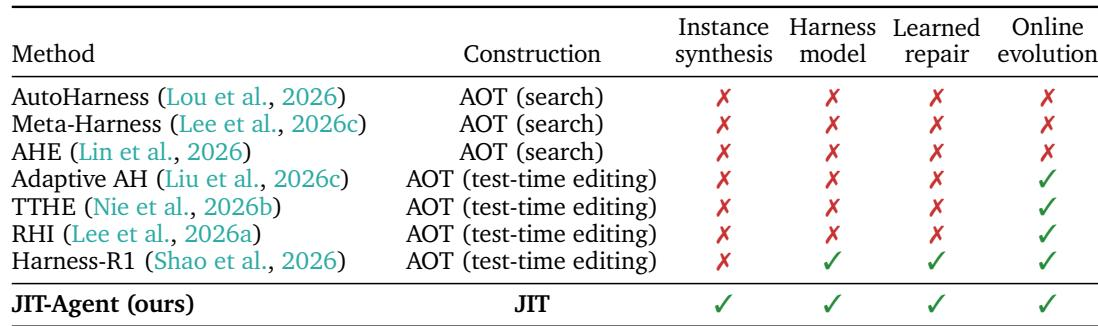
The table categorizes harness optimization methods by their construction paradigm, distinguishing between ahead-of-time search, ahead-of-time editing with test-time feedback, and just-in-time generation. It also tracks whether each method supports instance synthesis, trains a harness model, learns from failed executions, and continues evolving after deployment. The methods vary widely, with only the just-in-time approach combining all four capabilities. Ahead-of-time search methods lack instance synthesis, learned repair, and online evolution. Ahead-of-time editing methods add online evolution but still do not synthesize instances or train a harness model. The just-in-time approach is the only one that directly synthesizes instance-specific harnesses, trains the generator, learns from failed trajectories, and continues improving after deployment.
The seed bank contains 13 hand-written harnesses that instantiate a four-module protocol, covering heterogeneous memory, planning, action, and capability orchestration strategies. These harnesses serve as the initial population for synthesis and evaluation, with the bank expanding over time to include task-specific performance data. The harnesses vary in memory strategies, from full history to retrieval-based or reasoning-graph approaches. Planning modules range from no explicit planner to linear roadmaps, DAG planning, and dynamic decomposition. Action strategies include standard ReAct, marker-guided execution, and multi-rollout aggregation, while all harnesses share a full capability registry. The seed bank is designed to grow by retaining harnesses that advance the archive frontier, associating each with task, reward, latency, and cost.
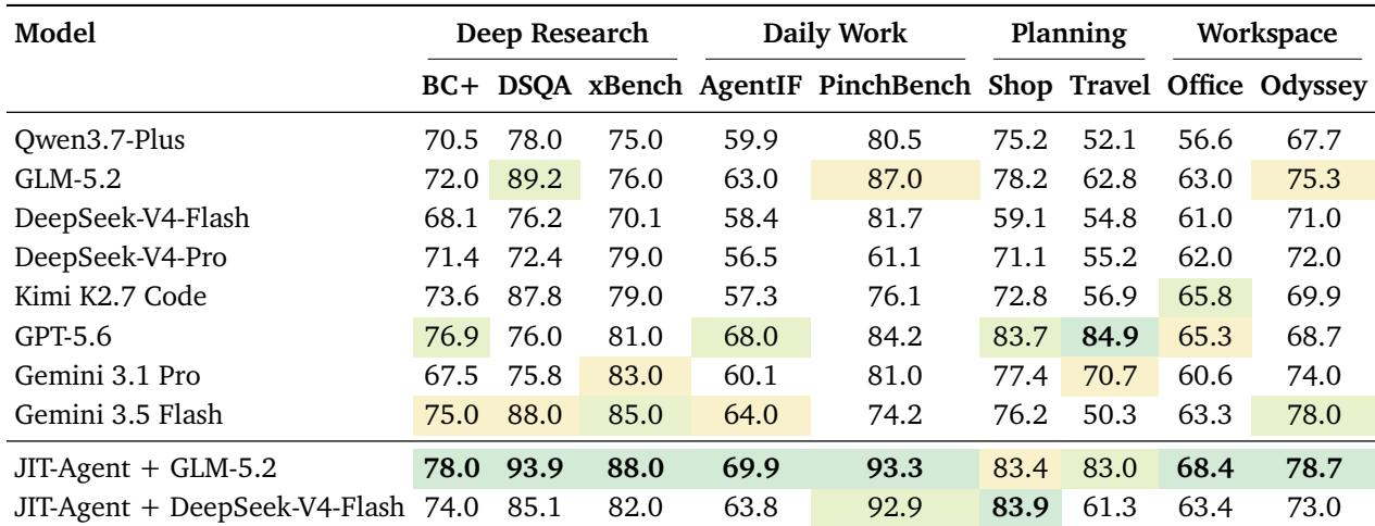
Replacing default scaffolds with JIT-generated harnesses consistently improves performance across all matched backbone-benchmark pairs, with average gains of 7.7 to 8.8 points on two backbones. The largest improvements occur on tasks requiring sustained state management and constraint tracking, and JIT-equipped systems achieve top results on eight of nine benchmarks, often surpassing stronger frontier models. JIT-generated harnesses improve performance on every matched backbone-benchmark pair, with average gains of 7.7 to 8.8 points. The largest gains are on planning tasks, with improvements of 24.8 and 20.2 points for DeepSeek-V4-Flash and GLM-5.2, respectively. JIT-equipped systems rank first on eight of nine benchmarks, with GLM-5.2 leading seven and DeepSeek-V4-Flash leading one. JIT-Agent with DeepSeek-V4-Flash exceeds the stronger DeepSeek-V4-Pro baseline on every reported benchmark, with an average advantage of 8.7 points. The only benchmark not led by a JIT-equipped model is DeepPlanning-Travel, where the JIT-equipped GLM-5.2 comes within 1.9 points of GPT-5.6.
A controlled comparison of advanced agent harnesses shows that generated harnesses like JIT-Agent often achieve better task performance with lower token usage and API cost than fixed harnesses across multiple backbones. The trade-offs vary by task, with some fixed harnesses remaining competitive on specific benchmarks, but the generated harness generally provides a more favorable cost-performance frontier. JIT-Agent outperforms all fixed harnesses on DeepSearchQA with the DeepSeek-V4-Flash backbone, achieving the highest performance while using the fewest tokens and lowest cost. On AgentIF, JIT-Agent improves performance over NanoBot while reducing cost, whereas NanoBot remains the best performer on xBench-DS for the same backbone. For Qwen3.6-Flash, JIT-Agent offers a lower-cost operating point with a modest performance trade-off compared to NanoBot, cutting cost by over half for a small performance drop.
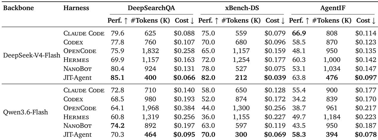
The evaluation compares harness optimization methods across construction paradigms, showing that only the just-in-time approach combines instance synthesis, trained harness models, learning from failed executions, and post-deployment evolution, while ahead-of-time methods lack key capabilities. A seed bank of 13 hand-written harnesses, covering diverse memory, planning, and action strategies, serves as the initial population and grows by retaining frontier-advancing harnesses. Replacing default scaffolds with JIT-generated harnesses yields consistent performance gains across backbones and benchmarks, with the largest improvements on planning tasks, and JIT-equipped systems often surpass stronger baselines. Cost-performance comparisons show that JIT-generated harnesses frequently achieve better task performance with lower token usage and cost than fixed harnesses, though trade-offs vary by task and backbone.