Command Palette
Search for a command to run...
Skaling: Chinchilla’s Exponents Meet Kaplan’s Coupling
Skaling: Chinchilla’s Exponents Meet Kaplan’s Coupling
Mathurin Videau Badr Youbi-Idrissi David Lopez-Paz Kartik Ahuja
Abstract
Neural scaling laws are foundational for language model development, yet standard formulations systematically underand overestimate loss at data-scarce and overtraining extremes. This failure originates in the underlying assumption that model size and training data impact the loss independently. To address this, we introduce the Skaling law (/"skeIlIN/), a generalized functional form that couples model capacity and data through a single interaction exponent. This simple extension reduces the Mean Absolute Percentage Error (MAPE) by 1.5–3× across both interpolation and extrapolation regimes. When paired with a sparse grid strategy restricted to low-compute regimes, the Skaling law achieves accurate full-grid extrapolation using approximately 10× less compute than uniform sweeps. By enabling reliable performance prediction from small-scale experiments, the Skaling law provides a more robust and resource-eficient framework for allocating compute budgets in next-generation model training.
One-sentence Summary
FAIR at Meta propose the Skaling law, a generalized neural scaling formulation that couples model capacity and data through a single interaction exponent, reducing MAPE by 1.5–3× across regimes and enabling accurate full-grid extrapolation from low-compute sparse grids using approximately 10× less compute than uniform sweeps.
Key Contributions
- The Skaling law introduces a generalized functional form that couples model capacity and training data through a single interaction exponent, correcting the independence assumption in standard additive scaling laws.
- This single-parameter extension reduces the Mean Absolute Percentage Error (MAPE) by 1.5–3× across both interpolation and extrapolation regimes and outperforms richer nine-parameter formulations at grid boundaries.
- Pairing the Skaling law with a sparse, L-shaped grid of low-compute boundary runs enables accurate full-grid extrapolation using approximately 10× less compute than uniform sweeps.
Introduction
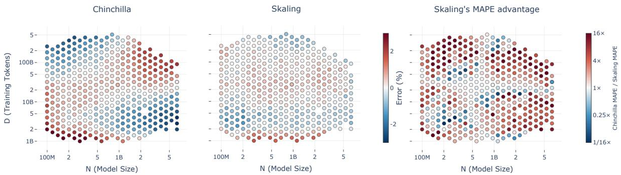
The predictable scaling of language model performance with model size and training data is essential for making cost-effective decisions about pretraining budgets and architectures. Widely adopted additive scaling laws, such as the Chinchilla formulation, treat the contributions of model size and data volume as independent terms, which forces their cross-derivative to zero and creates biased loss predictions at the boundaries of the training grid where the two are most imbalanced. The authors introduce the Skaling law, a minimal extension that adds a single coupling exponent to capture the interaction between model size and data, correcting boundary errors and enabling accurate scaling predictions from cheap L-shaped profiling grids that require up to 10× less compute.
Method
The authors begin by analyzing the loss surface to determine if model size (N) and training data (D) interact. They estimate derivatives using a Moving Least Squares (MLS) estimator. While first-order diagnostics suggest near-separability, the mixed derivative ∂2L/∂N∂D serves as the decisive test. An additive law requires this mixed derivative to be zero. However, the estimated mixed derivative is non-zero across the grid, exhibiting a power-law decay.
As shown in the figure below:
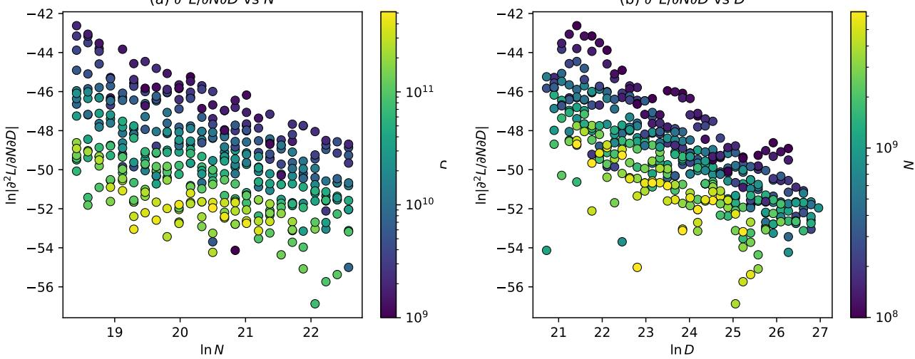
This non-zero mixed derivative indicates a synergy where scaling N and D together lowers loss more than scaling either alone, motivating a coupled functional form. The authors introduce the Skaling form:
L(N,D)=(NαA+DβB)k+EThis form bridges the additive Chinchilla law (recovered when k=1) and the coupled Kaplan form. By using a single outer exponent k while preserving independent inner exponents α and β, Skaling captures the interaction without tying the per-axis decay rates. It remains strictly decreasing and retains a closed-form compute-optimal allocation similar to the additive law, though the optimal ratio differs due to fitted parameters.
To estimate parameters efficiently, the authors avoid dense full-grid sampling, which is dominated by expensive large-scale runs. Instead, they employ an L-shape sampling strategy. This involves sweeping data volume D for the smallest models to isolate data parameters, and sweeping model size N for the shortest training horizons to isolate size parameters.
For evaluation, a comprehensive cross-validation framework is used. The data is partitioned into validation (interpolation), Extrapolation N (larger models), Extrapolation D (more data), and Far Extrapolation (largest models and data). Performance is measured using Mean Absolute Percentage Error (MAPE) across all sets and the coefficient of determination (R2) for interpolation.
To test predictive capability for massive pretraining runs, which typically scale along a fixed token-to-parameter ratio, the authors perform compute extrapolation along iso-ratio slices.
Refer to the framework diagram:
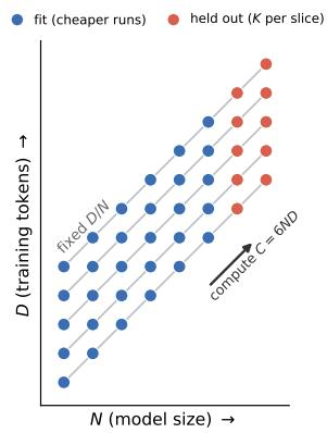
Runs are grouped into slices of constant D/N. Within each slice, the highest-compute points are held out. Scaling laws are fitted on the pooled low-compute points across all slices and evaluated on the held-out high-compute runs. This setup tests if a globally fitted law can predict expensive runs using cheap data, comparing against a per-ratio baseline that fits a one-dimensional power law within each slice.
Experiment
The evaluation uses two pretraining loss grids (Farseer and SK-Grid) and a cross-validation protocol that tests interpolation, single-axis extrapolation, and far extrapolation beyond the training boundaries. The Skaling law consistently reduces boundary errors compared to additive baselines, especially in imbalanced corners and sparse profiling regimes, because its coupled functional form captures the saddle-shaped interaction between model size and data. Compute extrapolation along fixed token-to-parameter ratios further shows that Skaling predicts high-cost runs from low-cost data more accurately and stably than global baselines, while the direction of the optimal allocation trend depends on the dataset and architecture. Overall, the results demonstrate that a multiplicative coupling between model and data scales provides better predictive accuracy and more reliable extrapolation than purely additive formulations.
The Skaling law dramatically reduces extrapolation error compared to the additive Chinchilla law, especially at grid boundaries and in far-extrapolation regimes, while achieving comparable or better interpolation fit. Sparse training on an L-shaped grid preserves Skaling’s accuracy but causes Chinchilla’s error to surge, demonstrating that high interpolation R² alone is insufficient to validate a scaling law. On the full SK-Grid, Skaling lowers far-extrapolation MAPE from 5.17% to 0.70%, and on the L-shape grid from 14.63% to 1.15%. Chinchilla attains strong interpolation R² (0.992–0.995) yet its extrapolation errors are several times larger than Skaling’s, showing that interior fit quality does not guarantee boundary accuracy.
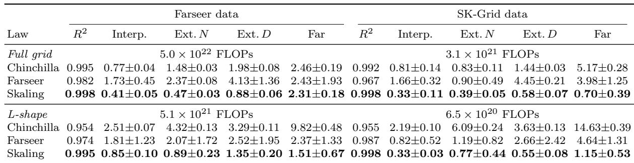
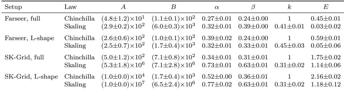
Fitting results show the Skaling law consistently recovers a sub-unit coupling exponent (k ≈ 0.31–0.45) instead of collapsing to the additive Chinchilla case (k=1), and its fitted irreducible loss is systematically lower, nearly vanishing on Farseer data. The coupling exponent and irreducible loss trade off against each other, allowing the coupled form to absorb curvature that the additive law would otherwise represent through a larger floor. This stable coupling explains why Skaling improves boundary predictions while remaining close to Chinchilla when the data are nearly additive. Across all grids the Skaling law fits a coupling exponent k between roughly 0.31 and 0.45, far from the additive value of 1. On Farseer data the fitted irreducible loss E drops from 0.45–0.59 under Chinchilla to 0.03–0.05 under Skaling, while on SK-Grid it remains substantial (1.14–1.75). With k < 1 the concave outer map makes the coupled reducible term decay more slowly at large scale, absorbing curvature that the additive law can only capture through a larger E.
The Skaling law consistently achieves the lowest prediction error across all training regimes when extrapolating to high-compute runs, with a pooled MAPE of 0.60%. Chinchilla’s error hides a severe drop in the optimal regime (3.47%), while the per‑ratio power law is competitive only near the optimum but cannot guide joint parameter–data allocation because it is fit separately within each slice. The more heavily parameterized Farseer law remains less accurate than Skaling overall. Skaling reduces extrapolation error nearly fourfold over Chinchilla and keeps MAPE below 0.9% in every regime, whereas Chinchilla exceeds 3.4% in the optimal band. The per‑ratio power law edges Skaling only in the optimal slice (0.77% vs 0.88%), but it is fit per recipe and cannot inform joint scaling decisions.
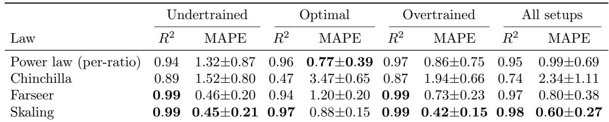
The Skaling law substantially reduces extrapolation error relative to the additive Chinchilla law, particularly at grid boundaries and in far-extrapolation regimes, while maintaining comparable interpolation fit. Sparse L-shaped training reveals that high interpolation R² is insufficient for validating a scaling law, as Chinchilla’s error surges under these conditions whereas Skaling remains accurate. Fitting results show that Skaling consistently recovers a sub-unit coupling exponent (k ≈ 0.31–0.45) and a systematically lower irreducible loss, allowing the coupled form to absorb curvature that the additive law would otherwise represent through a larger floor. Across all training regimes, Skaling achieves the lowest prediction error when extrapolating to high-compute runs, reducing error nearly fourfold over Chinchilla and keeping MAPE below 0.9% in every regime.