Command Palette
Search for a command to run...
House Price Calculation Methods for Beginners
Abstract
One-sentence Summary
By estimating a factor-augmented vector autoregression (FAVAR) model with Bayesian Normal-Gamma shrinkage priors and identifying monetary policy shocks via high-frequency surprises, this study analyzes monthly metropolitan home price data to reveal sizeable positive effects on regional housing prices that vary in magnitude and duration, with the largest impacts concentrated in California, Arizona, and Florida.
Key Contributions
- The study implements a factor-augmented vector autoregression (FAVAR) model estimated through a full Bayesian framework that applies Gibbs sampling and Normal-Gamma shrinkage priors to simultaneously recover latent factors and autoregressive coefficients.
- Monetary policy shocks are identified using high-frequency surprises around policy announcements as external instruments, which isolates exogenous policy changes without imposing restrictive structural assumptions.
- Empirical analysis of monthly housing price data across 417 US metropolitan regions over a 72-month horizon demonstrates substantial spatial heterogeneity, with the strongest positive effects concentrated on the East and West Coasts and high levels of local spatial autocorrelation.
Introduction
Understanding how national monetary policy influences regional housing markets is critical for economic forecasting and targeted policy design. Prior research typically relies on rigid structural models that impose theoretical constraints or standard vector autoregressions that lack robust uncertainty quantification and often aggregate data at the state level. The authors leverage a factor-augmented vector autoregression model combined with full Bayesian estimation to analyze monthly housing prices across 417 US metropolitan areas. By using high-frequency surprises around policy announcements to identify monetary shocks, they capture spatial heterogeneity and quantify parameter uncertainty, revealing that expansionary policy drives significant but geographically varied housing price responses over a multi-year horizon.
Dataset

-
Dataset Composition and Sources: The authors assemble a monthly panel dataset spanning April 1997 to June 2012 to analyze regional monetary policy transmission. Housing valuations come from the Zillow Home Value Index, national economic indicators are sourced from the FRED database, and credit spread metrics are drawn from the Gertler and Karadi (2015) archive.
-
Subset Details: The regional subset comprises 417 core-based statistical areas, filtered from an initial pool of 917 based on longitudinal data availability. This includes 264 metropolitan and 153 micropolitan regions. The national aggregate subset tracks seven variables: housing starts, the industrial production index, the consumer price index, the one-year government bond rate, the ten-year treasury minus federal funds rate spread, the prime mortgage spread over ten-year bonds, and the Gilchrist-Zakrajšek excess bond premium.
-
Data Usage: The authors structure the regional housing price vector and national aggregate vector as a simultaneous panel for macroeconomic modeling. This configuration allows them to isolate how national monetary policy and credit conditions drive divergent housing price responses across different geographic markets, rather than using traditional machine learning training splits or mixture ratios.
-
Processing and Adjustments: The authors seasonally adjust all series where applicable and apply mathematical transformations to achieve approximate stationarity. The Zillow index relies on statistical valuation models instead of repeat sales methods, capturing fair market values for all residential property types. The fixed 1997 to 2012 timeframe acts as the effective cropping strategy, ensuring uniform temporal coverage and metadata consistency across all 417 selected regions.
Method
The authors leverage a factor-augmented vector autoregressive (FVAR) model to analyze regional housing price dynamics, incorporating both latent common factors and observable macroeconomic aggregates. The framework is structured around two main equations: a measurement equation and a state equation. The measurement equation links observed housing prices Ht and national aggregates Mt to latent factors Ft and the observed aggregates, expressed as:
HtMt=ΛF0K×SΛMIKFtMt+ϵt0K×1,where Ft is an S×1 vector of unobserved latent factors capturing co-movement across regions, and Mt is a K×1 vector of observable national aggregates. The factor loadings matrices ΛF and ΛM map the factors and aggregates to regional housing prices, while ϵt represents region-specific measurement errors with diagonal variance-covariance matrix Σϵ. The identification of the model is achieved by constraining the upper S×S submatrix of ΛF to be the identity matrix IS, and setting the first S rows of ΛM to zero.
The evolution of the factors and aggregates is governed by a VAR process of order Q, specified as:
yt=Axt+ut,where yt=(Ft′,Mt′)′, xt=(yt−1′,…,yt−Q′)′, and A is a (S+K)×Q(S+K) coefficient matrix. The shocks ut follow a normal distribution with zero mean and variance-covariance matrix Σu. The parameters ΛF, ΛM, A, and the latent factors Ft are unknown and must be estimated.
To address the high dimensionality of the model, the authors adopt a Bayesian estimation framework. They stack the free elements of the factor loadings into a vector λ of length L=R(S+K) and the VAR coefficients into a vector a of length J=(S+K)2Q. Prior distributions are specified hierarchically to incorporate shrinkage and prior information. For the VAR coefficients aj, a Normal-Gamma shrinkage prior is employed, where each coefficient is conditionally normal with mean zero and variance proportional to a local scale τaj2, and the global shrinkage parameter ξa controls the overall degree of shrinkage. The local scales τaj2 and the global parameter ξa are assigned Gamma priors, allowing for a balance between sparsity and robustness to large deviations. The marginal prior on aj exhibits heavy tails, enabling the model to accommodate large effects when necessary. The variance-covariance matrix Σu is assigned an inverted Wishart prior to ensure proper shrinkage and posterior propriety.
For the factor loadings λℓ, a similar Normal-Gamma prior structure is used, with a single global shrinkage parameter ξλ applied across all loadings. This ensures that the factor loadings are shrunk toward zero while allowing for flexibility in individual elements. The measurement error variances σr2 are assigned independent inverted Gamma priors, with hyperparameters set to minimize prior influence. The estimation is conducted using a Markov Chain Monte Carlo (MCMC) algorithm, specifically Gibbs sampling, with 20,000 draws and a burn-in period of 10,000 draws. The model is implemented with Q=2 lags, and the number of latent factors S is selected using the deviance information criterion, resulting in S=1. Hyperparameters are set to induce strong shrinkage: ϑa=ϑλ=0.1, and c0=c1=d0=d1=0.01. The prior on Σu is weakly informative, with ν=S+K+1 and Σ=10−2IS+K, while the inverted Gamma priors on σr2 are set with e0=e1=0.01.
To achieve structural identification, the model incorporates high-frequency surprises in the three-months-ahead futures rate as an exogenous instrument for monetary policy shocks. This approach, adapted from Paul (2018), integrates the surprise variable zt into the state equation:
yt=Axt+ζzt+ut,where ζ is a vector of coefficients capturing the impulse response of the system to the monetary policy shock. This identification strategy avoids the need for zero restrictions and allows for consistent estimation of contemporaneous impulse responses. Higher-order responses are derived recursively using the state space representation of the VAR model.
Experiment
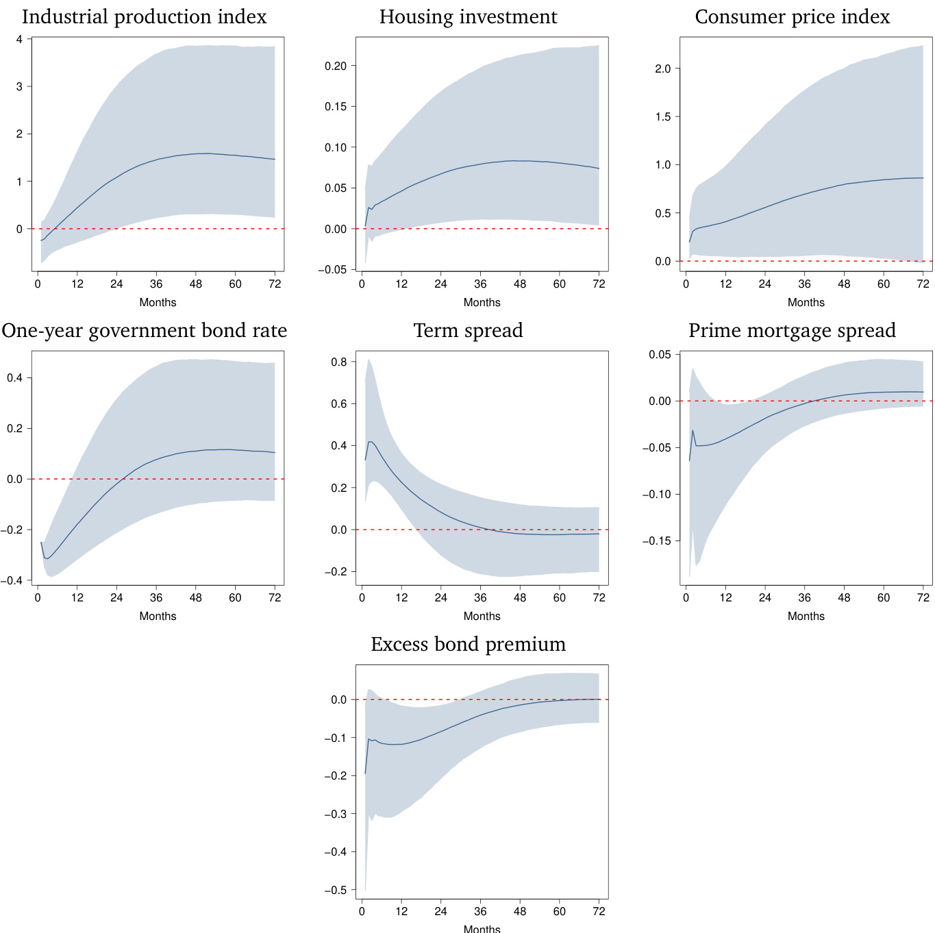
The study employs a Bayesian factor vector autoregression model using high-frequency policy surprises to identify monetary shocks and evaluates their dynamic impact on national macroeconomic fundamentals, a latent housing factor, and a broad panel of regional markets. This setup validates that expansionary policy consistently stimulates real economic activity and aggregate housing prices in line with established theory, while the latent factor successfully captures national price co-movement driven primarily by western and southern coastal states. Qualitatively, the regional analysis reveals substantial heterogeneity, with coastal areas experiencing the strongest and most persistent positive price effects while inland regions show muted or negative reactions. Furthermore, the findings demonstrate pronounced spatial dependence, indicating that neighboring regions exhibit highly similar dynamic responses, though the linear transmission framework may require nonlinear extensions to fully capture turbulent economic periods.