One-sentence Summary

Osaka University and University of Hildesheim propose FPMC, a method that unifies matrix factorization and personalized Markov chains by factorizing a user-specific transition cube via a Tucker-decomposition-based pairwise interaction model, subsuming both the common Markov chain and standard matrix factorization, adapting BPR for sequential basket data, and empirically outperforming both approaches.

Key Contributions

• The paper introduces FPMC, a recommender model that integrates matrix factorization and Markov chains by learning a personalized transition matrix for each user, forming a transition cube that captures both general user taste and recent sequential behavior.

• The method makes personalized transition graphs practical by factorizing the transition cube with a pairwise interaction model, a special case of Tucker decomposition, and adapts the Bayesian Personalized Ranking framework to learn from implicit sequential basket data.

• The work shows that FPMC subsumes common matrix factorization and nonpersonalized factorized Markov chains, while experiments on real-world data show FPMC outperforms MF, FMC, and unpersonalized MC on sparse and dense data.

Introduction

Recommender systems are important in e-commerce and web personalization because they use user activity data to predict what a user may buy next, helping increase sales, click-through rates, and user satisfaction. Prior methods typically chose between sequential Markov-chain models, which capture next-item behavior from recent purchases but share one transition pattern across users, and factorization models, which learn long-term user taste from all history but ignore sequence effects; direct estimation of user-specific transition matrices is also unreliable under sparse basket data. The authors leverage factorized personalized Markov chains, or FPMC, by assigning each user a personalized transition matrix and estimating the resulting transition tensor through low-rank factorization extended with Bayesian Personalized Ranking for basket data. This approach combines sequential behavior with user-specific taste and generalizes both standard Markov-chain and matrix-factorization recommenders.

Dataset

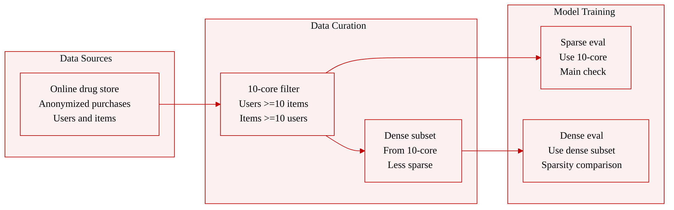
• The dataset is anonymized purchase data from an online drug store.

• The main evaluation set is a 10-core subset, constructed by filtering interactions so that:

  • every user has purchased at least 10 items in total, and
  • every item has been purchased by at least 10 users.

• The authors also create a denser subset from the 10-core dataset to study the effect of sparsity on the evaluated recommender methods.

• Dataset statistics are reported in Table 1 of the paper.

• The data is used to evaluate the recommender, with the 10-core subset representing the sparse setting and the denser subset used for comparison.

• The paper does not mention cropping, metadata construction, or other complex preprocessing beyond the 10-core filtering and creation of the dense subset.

Method

The authors address item recommendation from sequential set data. For each user $u$u, the observed behavior is a sequence of baskets

where $I$I is the item universe and each basket contains several items bought at the same relative time step. The target is to learn a personalized ranking over items for user $u$u at the next visit $t$t. Equivalently, the model induces an ordering

so that the top ranked items form the recommendation list.

Refer to the example below:

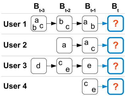
The basic building block is a Markov chain adapted to basket data. Because the state space of arbitrary subsets is $2^{|I|}$2∣I∣, a full chain over baskets is infeasible. The authors therefore model transitions at the item level and use first order dependencies. For any two items $l$l and $i$i, they define

which can be seen as an entry of an item transition matrix. Given the previous basket $B_{t-1}$Bt−1​, the probability that item $i$i appears in the next basket is averaged over all items in $B_{t-1}$Bt−1​:

This quantity is directly sortable, which makes it suitable for recommendation even though the true Markov chain over full baskets is not modeled explicitly.

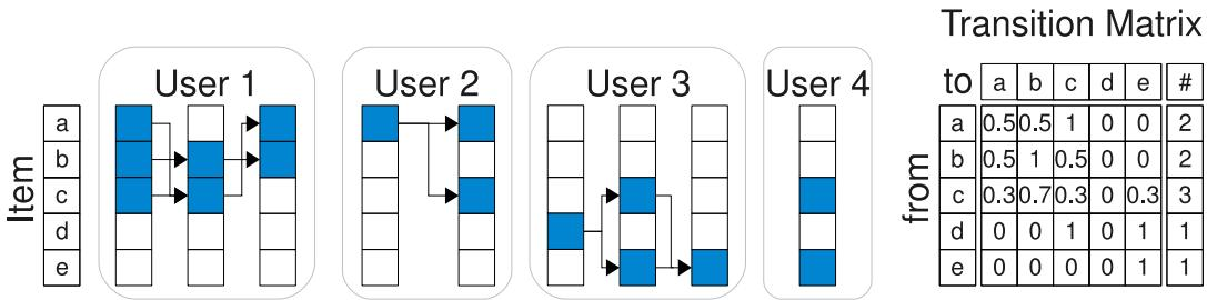
A maximum likelihood estimate for each item transition is obtained by counting observed basket pairs:

When personalization is added, the transition probability becomes user-specific:

forming a three-mode transition tensor $\mathcal{A} \in \mathbb{R}^{|U| \times |I| \times |I|}$A∈R∣U∣×∣I∣×∣I∣. The authors observe that this full parameterization is extremely sparse. Many transitions are never observed, and the observed ones often rest on very few counts, making maximum likelihood estimates unreliable. The transition matrix built from such counts is usually sparse and may favor popular but poorly ranked items. The following example illustrates a nonpersonalized transition matrix estimated by maximum likelihood:

To overcome this sparsity problem, the authors introduce the factorized personalized Markov chain, abbreviated as FPMC. The central idea is to replace the full transition tensor with a low rank approximation. They start from a Tucker style factorization:

where $V^U$VU captures user latent factors, $V^L$VL captures latent factors of items appearing in the previous basket, $V^I$VI captures latent factors of items to be predicted, and $\mathcal{C}$C is a core tensor. For sparse transition data, the authors use a more compact pairwise interaction form:

Each term has a clear interpretation. The first term captures a global user-item affinity, similar to standard matrix factorization. The second term captures transition affinity between the predicted item $i$i and an item $l$l from the previous basket. The third term captures user-conditioned transitions involving the previous basket.

The full personalized prediction for item $i$i given the previous basket is

Substituting the factorization gives

For item ranking, the $(U,L)$(U,L) interaction term is invariant under the pairwise ranking loss used in their training criterion. It depends on user $u$u and basket $B_{t-1}^u$Bt−1u​ but not on the candidate item being scored, so it cancels when comparing two candidate items. The authors therefore use the compact scoring function

This compact form shows the architecture as a joint extension of matrix factorization and a factorized Markov chain. The first term behaves like a personalized recommendation component, while the second term behaves like a sequential transition component. Unlike a simple ensemble of two separately trained models, all latent factors are learned together under the same ranking objective.

The training criterion is sequential Bayesian personalized ranking, called S-BPR. The authors optimize parameters $\Theta = \{V^{U,I}, V^{I,U}, V^{I,L}, V^{L,I}, V^{U,L}, V^{L,U}\}$Θ={VU,I,VI,U,VI,L,VL,I,VU,L,VL,U} so that items actually purchased in basket $B_t^u$Btu​ are ranked above items not present in that basket. Using the logistic sigmoid $\sigma(z)$σ(z), the ranking likelihood is

With Gaussian priors on the latent factors, the MAP objective becomes

Here $\lambda_\Theta$λΘ​ controls regularization, and the loss explicitly compares observed basket items $i$i against unobserved candidate items $j$j for the same user and time step.

Because the full set of quadruples $(u,t,i,j)$(u,t,i,j) is too large for direct optimization, the authors use bootstrap sampling with stochastic gradient descent. In each iteration, they sample one quadruple $(u,t,i,j)$(u,t,i,j), where $i$i is an item in basket $B_t^u$Btu​ and $j$j is an item not in that basket. They then update the model parameters using the gradient of the sampled S-BPR loss. For a scalar latent factor $\theta$θ, the update signal has the form

The model gradients couple the compact ranking scores to the underlying factor matrices. For example,

which means the user factor is updated according to the relative embedding difference between the observed and unobserved candidate items. The transition-related factors receive updates weighted by the average representation of the previous basket:

These update directions propagate information through user factors, candidate item factors, and previous basket item factors. The practical optimization loop samples one positive item, one negative item, one user, and one basket time step at a time, computes the sigmoid weighted gradient, and applies a gradient ascent step with regularization. The complexity per iteration is

where $k_{U,I}$kU,I​ and $k_{I,L}$kI,L​ are latent dimension sizes and $\overline{|B|}$∣B∣​ is the average basket size. This makes the bootstrap sampling procedure feasible for large item recommendation problems with sequential set behavior.

Experiment

Experiments evaluate factorized Markov chain recommenders on drug-store purchase data using a last-basket split and ranking metrics such as HLU, top-5 F-measure, and AUC, comparing them with dense MC, MF, and most-popular. Factorized models consistently beat the baselines, especially as data become sparse, because low-rank transition estimates densify sparse counts and reduce overfitting. MF performs relatively well on denser data, while MC and FMC benefit from sequential purchase signals in sparser settings, and FPMC combining both yields the strongest overall performance.

The experiments use anonymized online drug store purchase data from a sparse 10-core dataset and a dense subset built from the most active users and most purchased items. The dense subset has fewer users and items but more purchases per user, making it less sparse than the full dataset. Results from evaluations on these datasets show that factorized models improve over baselines and are especially useful in the sparse setting. The dense dataset focuses on active users and popular items to study sparsity effects. Sparse transition data makes factorized transition estimates more advantageous than direct counting.

The counting-based transition matrix is very sparse on the sparse dataset, while the dense dataset contains a much higher proportion of filled entries. This sparseness explains why factorized transition estimation can outperform standard counting, especially on sparse data, by densifying the matrix and reducing overfitting. Even in the dense setting, the factorized model still outperforms the counting-based model because it uses fewer parameters. Standard counting produces a sparse transition matrix on the sparse dataset and a much denser one on the dense dataset. Factorized transition estimation provides a clearer advantage when the counting-based matrix is sparse. The factorized model remains better than counting in the dense case by avoiding overfitting through low-rank estimation.

The experiments evaluate factorized transition models on anonymized online drug store purchase data using a sparse 10-core dataset and a denser subset focused on active users and popular items. The results show that factorized models consistently improve over baseline counting-based approaches, with the strongest benefit in sparse settings where transition matrices are too sparse for reliable direct estimation. By densifying transition estimates and reducing overfitting through low-rank modeling, factorized approaches remain advantageous even in the denser dataset.