One-sentence Summary

NVIDIA, MIT, and UIUC propose MOTIVE, the first motion-centric gradient-based data attribution framework for video generation that isolates temporal dynamics from static appearance via motion-weighted loss masks, enabling scalable influence computation to curate fine-tuning data that improves temporal consistency and physical plausibility.

Key Contributions

• This work presents MOTIVE, a motion-centric gradient-based data attribution framework for video generative models that attributes fine-tuning clips to temporal dynamics rather than static visual appearance at large modern video scales.

• MOTIVE uses motion-weighted loss masks to isolate temporal dynamics from static appearance, enabling efficient motion-specific influence computation and identification of clips that strongly affect motion smoothness, temporal consistency, and physical plausibility.

• Experiments on text-to-video models show that MOTIVE-guided data curation improves motion smoothness and dynamic degree on VBench, achieving a 74.1% human preference win rate against the pretrained base model.

Introduction

Video generation with diffusion or flow-matching models goes beyond image synthesis because it must learn temporal dynamics such as object motion, camera movement, deformation, and physical interaction. As these models scale with data, understanding which training clips teach a model to move well is important for diagnosing artifacts and selecting fine-tuning data, especially when large pretraining corpora are unavailable.

Existing data attribution methods mainly explain static visual content and, when applied naively to videos, conflate appearance with motion. They can fail to localize dynamic regions, become costly when integrating gradients across frames, and suffer from biases such as clip length or diffusion timestep effects.

The authors leverage gradient-based attribution to build MOTIVE, a motion-aware framework that masks toward dynamic regions, corrects frame-length effects, and traces generated motion to influential training clips. It also uses efficient approximations to scale to large models and datasets, and it can improve motion smoothness and dynamic degree with a small fraction of training data.

Method

The authors design an attribution framework for video diffusion models in the fine-tuning setting. The input is a fine-tuning corpus $\mathcal{D}_{\mathrm{ft}} = \{(\mathbf{v}_n, \mathbf{c}_n)\}_{n=1}^{N}$Dft​={(vn​,cn​)}n=1N​ and a query video-caption pair $(\hat{\mathbf{v}}, \hat{\mathbf{c}})$(v^,c^). The goal is to assign each training clip $(\mathbf{v}_n, \mathbf{c}_n)$(vn​,cn​) a motion-aware influence score that explains how that clip contributes to the temporal dynamics observed in the generated query video. The design is guided by two practical constraints: the score should be predictive of which data subsets actually improve target motion during fine-tuning, and it should scale to large video models and large corpora without requiring inverse Hessian inversion, per-example trajectory integration, or full gradient storage.

The pipeline converts attribution into a compact gradient geometry problem. Instead of estimating the exact curvature involved in classical influence functions, the authors approximate the inverse Hessian with an identity preconditioner and estimate influence from the alignment of training and test gradients. The diffusion loss gradients are computed under paired random variables, so the same timestep and noise vector are used for both the training clip and the query clip. This shared randomness reduces variance and makes the ranking of candidate examples more stable.

For a set of sampled noise-timestep pairs $\mathcal{T}$T, a paired multi-sample estimator can be written as

To reduce cost further, the framework collapses this into a single-sample estimator by fixing one shared timestep $t_{\mathrm{fix}}$tfix​ and one shared noise draw $\boldsymbol{\epsilon}_{\mathrm{fix}} \sim \mathcal{N}(\mathbf{0}, \mathbf{I})$ϵfix​∼N(0,I) across all query-training comparisons. The resulting cosine-like score is

Because raw gradients are prohibitive to store for billion-parameter video models, the method adds a structured random projection step. A Johnson-Lindenstrauss style Fastfood projection maps high-dimensional gradients into a smaller space while preserving relative cosine geometry. The projection matrix is constructed from a sequence of randomized transforms,

where $\mathbf{Q}$Q is a Walsh-Hadamard matrix, $\mathbf{B}$B is a diagonal Rademacher matrix, $\Pi$Π is a random permutation, $\mathbf{G}$G is a diagonal Gaussian scaling matrix, $\mathbf{S}$S is a diagonal rescaling matrix, and $\xi$ξ stabilizes the variance. Each gradient is projected and then normalized,

The final video-level score is the cosine similarity in the projected space,

This gives approximate gradient similarity while storing only low-dimensional vectors per example.

The authors also correct a video-specific scale problem. Raw diffusion gradients grow with the number of frames $F$F in a video, which can bias rankings toward longer clips. To remove this length-dependent inflation, the gradient is divided by the frame count before projection and normalization:

The framework then still applies $L_2$L2​ normalization to stabilize comparisons across clips.

Video-level gradient similarity alone is not sufficient for motion understanding because it can reward shared appearance, backgrounds, or objects rather than temporal dynamics. The central module of the method is therefore motion attribution. This module operates in the latent space used by the video diffusion model. Given a video

the encoder maps it to latent features

with a spatial downsampling factor $s$s and latent channel dimension $C$C. In the described implementation, the latent geometry matches a video VAE backbone with $s=8$s=8 and $C=16$C=16.

Motion information is computed in pixel space using a dense motion tracker or optical flow extractor. The tracker produces

where the first two channels encode horizontal and vertical pixel displacement between frames, while the remaining channels encode visibility or confidence information. The displacement vector at frame $f$f and pixel location $(h,w)$(h,w) is

The raw motion magnitude is the Euclidean norm

To avoid dominance from videos with unusually large absolute motion magnitudes, these values are min-max normalized across all frames and pixel locations:

where

and $\zeta = 10^{-6}$ζ=10−6 prevents division by zero. This normalization emphasizes relative motion saliency rather than raw displacement scale.

The motion weights are then bilinearly downsampled from pixel resolution to the latent grid:

Using fixed $t_{\mathrm{fix}}$tfix​ and $\boldsymbol{\epsilon}_{\mathrm{fix}}$ϵfix​, the method computes a per-location squared error between the predicted noise and the target noise at each latent frame and latent spatial location:

The motion-weighted attribution loss is the average of these errors weighted by the latent-aligned motion mask:

The factor $1/F_{\mathbf{v}}$1/Fv​ again removes frame-length bias. When the motion weights are all equal to one, the objective reduces to a standard averaged diffusion loss without motion emphasis.

The motion-aware gradient is then

and the projected and normalized motion gradient is

The final motion attribution score is

In practice, the candidate clip $(\mathbf{v}_n,\mathbf{c}_n)$(vn​,cn​) and query clip $(\hat{\mathbf{v}},\hat{\mathbf{c}})$(v^,c^) provide conditioning information to the diffusion model, while the motion mask determines which latent error locations dominate the attribution gradient. Because masking is applied in the attribution loss rather than in forward noising or generation, the diffusion model itself is not altered. The motion-weighted gradient instead shifts the attribution objective toward dynamic regions and away from static backgrounds.

The attribution scores are then used to construct fine-tuning subsets. For a single query clip and a budget $K$K, the framework selects the top-$K$K candidate examples by motion-aware score. In practical data selection, $K$K may be specified as a percentile of the candidate corpus, such as the top one to ten percent, so that the selected subset scales consistently across dataset sizes.

For multiple query motions, the framework aggregates scores across queries with a majority voting mechanism. For $Q$Q query clips, each query contributes a binary vote for a training clip if that clip’s motion-aware score exceeds a percentile cutoff $\tau$τ for that query. The consensus vote count is

The final fine-tuning subset contains the top-$K$K examples with the largest $\mathrm{MajVote}_n$MajVoten​. This avoids the need to calibrate raw influence scores across different query motions, while still preferring clips that are repeatedly identified as motion-influential.

The computational design keeps the workflow tractable for large video corpora. Naive attribution that averages over many timesteps and noise samples would require cost proportional to the dataset size times the number of samples. The single fixed noise-timestep variant reduces gradient computation to one forward-backward pass per example. Projection adds a structured $\mathcal{O}(D'\log D')$O(D′logD′) cost per gradient, which is small relative to a diffusion model backward pass. Instead of storing full gradients of dimension $D$D, the system stores projected vectors of dimension $D'$D′, plus the compact randomized projection state. Candidate ranking then reduces to inner products in $\mathbb{R}^{D'}$RD′ and sorting. The motion mask extraction adds frame-resolution overhead, but the masks can be computed once per clip and cached, making their cost negligible relative to gradient computation.

Experiment

The experiments evaluate motion attribution for video generation fine-tuning using large-scale datasets, diverse motion-category queries, pretrained diffusion video models, automated VBench metrics, human preference studies, and ablations. Results show that the proposed attribution selects physically meaningful motion examples and improves generated motion fidelity and temporal dynamics over random, magnitude-based, embedding-based, and full-video baselines while preserving visual quality. Ablations further confirm that compact attribution settings, including a fixed denoising timestep, projected gradients, and frame-length normalization, retain ranking quality and reduce bias toward video length.

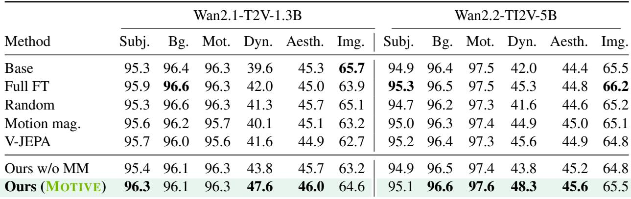
MOTIVE uses motion-aware attribution to select training data and shows the strongest VBench motion quality across both video models. It achieves the highest dynamic degree scores while also supporting strong aesthetic quality and competitive motion smoothness. These improvements come from selecting only a small training data fraction and exceed full fine-tuning on dynamic degree, highlighting the value of motion-specific data selection. MOTIVE reaches the highest dynamic degree across both evaluated models. It outperforms random selection and whole-video attribution on motion-oriented performance. Motion-guided selection with a small data budget surpasses full fine-tuning on dynamic degree.

Human evaluators generally preferred the attribution-guided video selection over the tested baselines. The preference was strongest against the base model and remained positive against random and full fine-tuned selection, though by narrower margins. Removing motion masking weakened the advantage, producing fewer clear wins and more ties. Strongest human preference appeared against the base model Perceptual advantage persisted against full fine-tuned selection Omitting motion masking increased ties and reduced clear wins

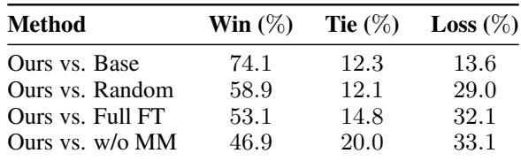
Experiments evaluate MOTIVE through automatic VBench and human preference tests across video models. They show that motion-aware attribution data selection yields the strongest dynamic motion quality while preserving aesthetic and smoothness results, and small selective budgets can outperform full fine-tuning. Human evaluations further confirm the perceptual advantage over baselines, especially versus the base model, while removing motion masking reduces the benefit.