One-sentence Summary

Google's Batch Normalization method normalizes each layer's inputs per mini-batch as part of the model architecture to mitigate internal covariate shift, enabling higher learning rates and achieving $4.82\%$4.82% top-5 ImageNet error with $14$14 times fewer training steps than prior state-of-the-art models.

Key Contributions

• Batch Normalization is introduced as a normalization mechanism for layer inputs within the model architecture for each training mini-batch, reducing instability from changing activation distributions and enabling higher learning rates, less careful initialization, and often no Dropout.

• An algorithm is provided for constructing, training, and performing inference with batch-normalized networks, including learned scale and shift parameters, support for convolutional layers, and deterministic inference that does not depend on mini-batch statistics.

• Applied to a state-of-the-art image classification model, Batch Normalization matches the original model's accuracy with 14 times fewer training steps and exceeds it, while an ensemble reaches 4.82% top-5 test error on ImageNet, improving the best published result.

Introduction

The authors study deep neural network training with stochastic gradient descent, where minibatches are used because they provide efficient gradient estimates and faster optimization on modern hardware.

A key limitation of prior approaches is that training remains sensitive to hyperparameters and initialization, and the input distribution to each layer changes during optimization. The authors call this internal covariate shift, which can slow convergence, amplify saturation in nonlinearities, and contribute to vanishing gradients.

To address this, the authors introduce Batch Normalization, which normalizes layer inputs within each minibatch and uses learnable scale and shift parameters to preserve representational capacity. This stabilizes activations, improves gradient flow, enables much higher learning rates, supports saturating nonlinearities, and accelerates training with lower dropout requirements.

Method

The authors focus on reducing internal covariate shift, which they define as the change in the distribution of activations within a network as training progresses. In standard deep networks, earlier layers continually modify their outputs as parameters are updated, forcing later layers to adapt to non-stationary input distributions. This can slow optimization, increase sensitivity to initialization, and make training unstable. The proposed method addresses this by inserting a normalization transformation into the network itself so that activations entering subsequent layers have more stable first and second moments throughout training.

The key design choice is to make normalization a differentiable part of the model rather than a separate preprocessing step applied outside the gradient computation. If normalization is applied after parameter updates but ignored during backpropagation, the optimizer may update parameters in a way that is immediately undone by the normalization step. For example, if a bias is updated and then a mean subtraction cancels the effect of that bias, the loss may remain unchanged while the bias grows. By embedding normalization into the forward computation, the network learns with knowledge of the transformation, and the optimizer can account for how parameter changes affect the normalized activations.

The method normalizes each scalar feature dimension independently. For a layer input vector $\mathbf{x} = (x^{(1)}, \dots, x^{(d)})$x=(x(1),…,x(d)), each dimension is standardized as

Instead of using full whitening, which would require computing and inverting covariance matrices and their derivatives, the method normalizes dimensions separately. This greatly reduces computational cost while still improving convergence. Full decorrelation is avoided because it requires expensive operations and can be unstable when estimated from minibatches whose size is smaller than the feature dimension.

A simple normalization step can limit the expressive power of a layer, especially when the normalized activations are passed through saturating nonlinearities such as the sigmoid. To preserve the representational capacity of the network, the normalized value is followed by a learned affine transformation:

Here, $\gamma^{(k)}$γ(k) and $\beta^{(k)}$β(k) are learned parameters that scale and shift each activation dimension. If the optimal representation requires the original unnormalized activations, the transformation can recover them by learning

Thus, the normalization does not force the network into a constrained family of functions. It provides a trainable mechanism that can restore the identity transformation if needed.

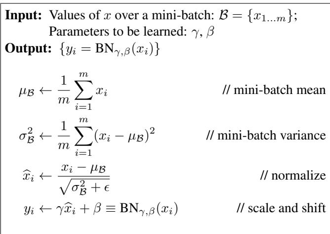
During stochastic training, the statistics used for normalization are computed over a minibatch. Consider a minibatch $\mathcal{B} = \{x_1, \dots, x_m\}$B={x1​,…,xm​} for one activation dimension. The batch mean and variance are

and

The normalized and transformed values are computed as

followed by

A small constant $\epsilon$ϵ is added to the variance for numerical stability. This transformation, often called the batch normalizing transform, maps the minibatch activations $\{x_i\}${xi​} to transformed activations $\{y_i\}${yi​}. Because the statistics are computed from the same minibatch used for optimization, the normalization participates directly in backpropagation. The gradients flow through the mean, variance, scaling parameter, and shift parameter, allowing the learning procedure to adjust the model in a way that is consistent with the normalization step.

The backward pass propagates the gradient through the normalization and affine transformation using the chain rule. Starting from the loss $\ell$ℓ, gradients first flow through the affine layer:

Gradients then accumulate into the batch statistics:

and

The gradient with respect to each input activation $x_i$xi​ is

The affine parameters receive gradients

and

This differentiability is central to the method. The normalized activations are not treated as fixed constants during optimization. Instead, they are embedded in the computational graph, which allows each layer to continue learning on input distributions with reduced internal covariate shift.

At inference time, the method changes from minibatch statistics to fixed population statistics. The normalized activation is computed as

where the mean and variance are estimated from training. These estimates can be accumulated during training using moving averages or unbiased estimators based on minibatch statistics. Since the inference-time mean and variance are fixed, the normalization becomes a simple linear operation. It can be combined with the learned scaling and shift parameters $\gamma$γ and $\beta$β into a single affine transformation. This makes deployment efficient and deterministic, because the output no longer depends on other examples in a batch.

When applied to standard layers of the form

where $g(\cdot)$g(⋅) is a nonlinear activation such as ReLU or sigmoid, the normalization is inserted before the nonlinearity. The transformed preactivation $\mathbf{x} = \mathbf{W}\mathbf{u} + \mathbf{b}$x=Wu+b is normalized. Because mean subtraction later removes any constant shift, the original layer bias $\mathbf{b}$b can be omitted. Its role is absorbed by the learned shift parameter $\beta$β. The resulting layer becomes

This placement is preferred over normalizing the layer inputs $\mathbf{u}$u directly. The distribution of $\mathbf{u}$u often changes during training because it may be produced by another nonlinearity, so constraining its mean and variance may not fully stabilize its higher-order shape. The preactivation $\mathbf{W}\mathbf{u}$Wu is more likely to have a symmetric and stable distribution, making normalization more effective.

For convolutional networks, normalization is adapted to respect convolutional structure. Instead of normalizing every spatial location independently, activations from the same feature map are normalized jointly across the minibatch and spatial locations. If the minibatch size is $m$m and each feature map has spatial size $p \times q$p×q, the effective batch size for a given feature map is

The learned parameters $\gamma^{(k)}$γ(k) and $\beta^{(k)}$β(k) are shared across spatial positions within a feature map rather than being learned separately for each location. This preserves translation equivariance and ensures that all activations in the same feature map undergo the same transformation.

The method also changes the optimization behavior of the network. By stabilizing activation distributions, it reduces the amplification of small parameter changes as signals propagate through many layers. This allows larger learning rates to be used more safely. The normalization transformation also makes training less sensitive to parameter scale. For a scalar $a$a,

because the normalization removes the global scaling. As a result, increasing the magnitude of $\mathbf{W}$W does not directly increase the gradient magnitude during backpropagation. Larger weights can even lead to smaller gradients with respect to the weight matrix, which helps control parameter growth. This behavior makes high learning rates more stable and reduces the risk of exploding or vanishing gradients.

The training process can be further adjusted to exploit the regularization effect of the normalization. Because each training example is normalized using statistics from its minibatch, its transformed representation depends on other examples randomly sampled in the same batch. This introduces a form of stochastic regularization. In practice, this allows the training configuration to rely less on other regularizers. The weight decay can be reduced, dropout can be removed in some architectures, and more aggressive learning rate schedules can be used. Since the network trains faster, training examples may be observed fewer times, and augmentation or photometric distortion can be reduced so that the model focuses more on naturally distributed examples. These adjustments reflect the central design of the method: normalization is not merely a preprocessing step, but an integral trainable module that stabilizes optimization, preserves model capacity, and reshapes the training dynamics.

Experiment

The experiments first use a simple MNIST model to show that Batch Normalization stabilizes hidden-layer activation distributions and improves test accuracy relative to a baseline. They then evaluate a modified Inception network on ImageNet, demonstrating that Batch Normalization combined with adjusted training settings accelerates optimization, increases attainable accuracy, and enables otherwise difficult sigmoid-based training. Finally, an ensemble of Batch Normalization-based models achieves state-of-the-art ImageNet classification performance.

The Batch Normalizing Transform standardizes activations using the mean and variance of a mini-batch, then applies learnable scaling and shifting. In the reported experiments, this reduces training difficulty and allows models to reach strong validation accuracy with far fewer steps. It also supports harder configurations, including higher learning rates and sigmoid nonlinearity. The baseline Batch Normalization model reaches the reference accuracy with less than half the training steps. A higher learning rate variant can train more slowly at first but reaches a higher final accuracy. With sigmoid activation, normalization enables meaningful accuracy where the original model remains near chance.

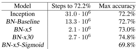
Batch normalization accelerates training and improves validation accuracy over Inception. The batch-normalized models reach Inception's 72.2 percent accuracy in far fewer training steps, with BN-x5 requiring the fewest steps and BN-x30 achieving the highest accuracy despite slower early convergence. Sigmoid becomes trainable with batch normalization but still performs below the ReLU variants. Batch normalization matches Inception accuracy in less than half the training steps BN-x5 reaches the 72.2 percent accuracy threshold fastest among the batch-normalized variants BN-x30 trades slower convergence for the highest maximum accuracy Sigmoid without batch normalization remains at chance accuracy

The table compares a batch-normalized Inception model with earlier ImageNet classification results. A single-crop BN-Inception model is reported near single Deep Image models in top-5 error, while the accompanying text says a BN-Inception ensemble reaches 4.9 percent top-5 error on the validation set and 4.82 percent on the test server. The ensemble result is presented as improving the previous best reported result. Ensembles of BN-Inception models are described as setting a new state-of-the-art result over prior reported top-5 errors. The single-crop BN-Inception result is weaker than the strongest ensemble results shown, indicating ensemble inference gives the main accuracy gain.

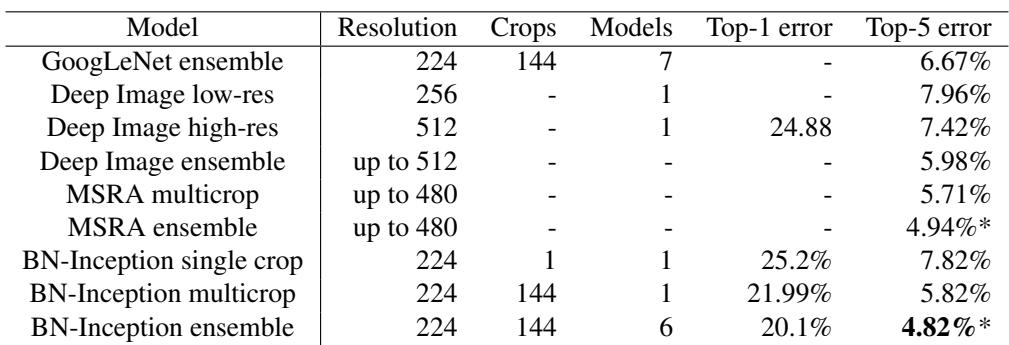
The experiments evaluate Batch Normalization in Inception-style ImageNet classifiers by comparing training convergence, final accuracy, activation choices, and results against earlier models. They show that normalization greatly eases optimization, accelerates training, supports higher learning rates, and makes sigmoid networks learnable. Batch-normalized variants also achieve competitive or improved accuracy, though some favor faster convergence while others favor higher final performance, and ensemble inference provides the strongest overall ImageNet gains.