One-sentence Summary

Researchers at Seoul National University, KTH Royal Institute of Technology, FleetMQ, and California Institute of Technology demonstrate the Autonomy Testbed for Multi-purpose Orbiting Systems (ATMOS), a planar spacecraft-analog robot for hardware-in-the-loop evaluation, and experimentally validate a control strategy that combines state prediction and trajectory tracking for docking under time-varying random communication delays, including an intercontinental Seoul-to-Stockholm teleoperation experiment.

Key Contributions

• The paper presents the Autonomy Testbed for Multi-purpose Orbiting Systems (ATMOS), a planar free-flying spacecraft-analog robot for hardware-in-the-loop evaluation of guidance and control strategies under microgravity-like conditions.
• A delay-aware control strategy combines state prediction against slowly varying, stochastic communication latency with a control Lyapunov function-based tracking controller to perform docking maneuvers under time-varying round-trip delays.
• A transcontinental closed-loop experiment between Seoul and Stockholm over a 7450 km link demonstrates stable remote docking under realistic intercontinental delay and variability, validating ATMOS as a rapid and cost-effective testbed for spacecraft teleoperation concepts.

Introduction

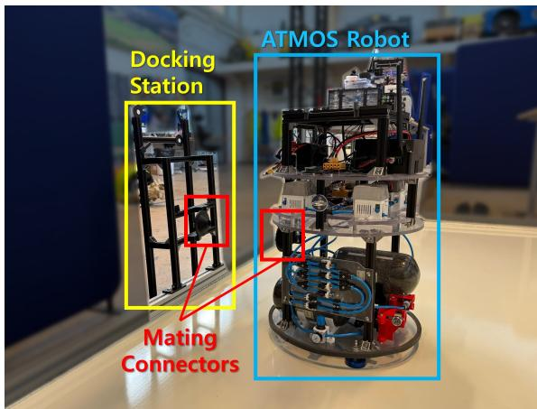
Space missions increasingly rely on remote-control and networked multi-agent architectures for terrestrial and extraterrestrial tasks, but these approaches depend on communication networks that can introduce delays, jitter, and packet loss, all of which can significantly degrade closed-loop performance. Validating delay-resilient control strategies safely on the ground requires experimental platforms that reproduce realistic communication conditions while enabling repeatable hardware-in-the-loop testing. The authors present the ATMOS planar free-flying space robot and develop a delay-aware Control Lyapunov Function based controller that tracks fixed and time-varying reference trajectories despite stochastic, time-varying communication delays. Their main contribution is a transcontinental closed-loop demonstration between Seoul and Stockholm over 7450 km, where control inputs and state measurements are exchanged through FleetMQ, and state prediction against observed latency is used to apply control in the direction that reduces the Control Lyapunov Function value.

Method

Control Methodology

The authors model ATMOS as a three-degree-of-freedom robotic platform that moves quasi-frictionlessly on a resin plate. Its configuration is described by $\boldsymbol{q}=(\boldsymbol{p},\psi)\in\mathbb{R}^2\times(-\pi,\pi]$q=(p,ψ)∈R2×(−π,π], where $\boldsymbol{p}$p is the robot position and $\psi$ψ is the yaw angle. The velocity twist is $\dot{\boldsymbol{q}}=[\boldsymbol{v}^\top\ \omega_z]^\top\in\mathbb{R}^3$q˙​=[v⊤ ωz​]⊤∈R3, with linear velocity $\boldsymbol{v}$v and angular rate $\omega_z$ωz​. The actuation wrench is $\boldsymbol{u}=[\boldsymbol{f}^\top\ \tau_z]^\top\in\mathbb{R}^3$u=[f⊤ τz​]⊤∈R3, consisting of body-frame force $\boldsymbol{f}$f and torque $\tau_z$τz​. The full nonlinear acceleration model is

with

where $m$m is the robot mass, $I_z$Iz​ is the inertia about the vertical axis, and $R_z(\psi)$Rz​(ψ) is the rotation matrix about the z-axis. Defining the state $\boldsymbol{x}=[\boldsymbol{q}^\top\ \dot{\boldsymbol{q}}^\top]^\top$x=[q⊤ q˙​⊤]⊤, the dynamics can be written in input-affine form as

where

The remote control architecture uses timestamped packet exchanges between the controller and the robot. The controller sends control packets $U_i=(\boldsymbol{u}_i,t_i^u)$Ui​=(ui​,tiu​), where $t_i^u$tiu​ is the controller-clock timestamp and $\boldsymbol{u}_i$ui​ is the commanded input. The robot returns state packets

where $\boldsymbol{x}_k$xk​ is the state measured at robot time $s_k^x$skx​, $i_k$ik​ is the index of the latest applied control packet, and $\Gamma_k=(\Delta_1,\dots,\Delta_{N_s})$Γk​=(Δ1​,…,ΔNs​​) is a list of recent control packet delay samples. The delay is defined as $\Delta_i=s_i^u-t_i^u$Δi​=siu​−tiu​, where $s_i^u$siu​ is the robot-clock arrival time of packet $U_i$Ui​. Lost and out-of-order packets are handled explicitly: if multiple packets are lost before the next successful arrival, they are treated as arriving simultaneously with that arrival, and a packet arriving later than a newer packet is discarded.

When the controller receives a state packet $X_k$Xk​, it computes a new control packet $U_k=(\boldsymbol{u}_k,t_k^u)$Uk​=(uk​,tku​). However, the state at which $U_k$Uk​ will actually be applied is unknown because of transmission delay and clock bias. The authors therefore estimate this future state by simulating the pending control packets. For each pending packet $U_j$Uj​, with $i_k+1\leq j\leq k$ik​+1≤j≤k, the predicted arrival time is

where $\hat{\Delta}_j$Δ^j​ is randomly sampled from the current delay list $\Gamma_k$Γk​. The input is assumed to be applied with zero-order hold, so that

The predicted state at the arrival of the current control packet is then obtained by integrating the system dynamics,

If the predicted arrival times violate their original order, meaning $\hat{s}_j^u\geq \hat{s}_{j+1}^u$s^ju​≥s^j+1u​, the corresponding packet is treated as lost. Repeating this prediction with $N$N different sampled delay profiles produces a particle set

which approximates the distribution of the state at which the newly computed control input will be applied.

For reference tracking, the authors use a control Lyapunov function $V(\boldsymbol{x};\boldsymbol{x}_{\mathrm{ref}})$V(x;xref​). If the exact future state $\boldsymbol{x}_k^+$xk+​ were known, the input could be selected to enforce the decrease condition

Because only the particle set $X_k^+$Xk+​ is available, the controller enforces this condition for all predicted particles. The control input is computed by solving

Here, $\delta$δ is a slack variable that relaxes the CLF decrease condition when strict satisfaction is not possible for all predicted states, and $p$p balances the reference input tracking objective against the CLF constraint satisfaction. A larger $p$p prioritizes robust enforcement of the CLF condition, producing a more conservative behavior. Since the dynamics are input-affine, this optimization is a quadratic program with linear constraints, and it is always feasible.

For the docking demonstration, the reference trajectory fed into the CLF controller is generated by a two-step motion planning strategy. First, the robot stabilizes to a parking configuration directly facing the docking station, with zero reference velocity. Once the robot is sufficiently close to the parking configuration, an online optimal control problem generates the docking trajectory. The yaw angle is always set to face the docking position and is not part of the optimization. The translational reference is obtained by solving

subject to the discrete-time double-integrator dynamics

the terminal docking condition

and time-varying acceleration limits

The acceleration limits are chosen as a decreasing function of the time index $k$k, reducing the effect of possible deviations from the docking trajectory caused by overly aggressive accelerations.

Experiment

The evaluation combines simulation and hardware experiments. Software-in-the-loop simulations test stabilization and circular trajectory tracking under stochastic delays and packet loss, showing that the proposed controller consistently improves position and yaw tracking accuracy over a naive PD reference controller, especially as delay severity increases. A hardware demonstration performs remote closed-loop docking of the ATMOS robot over an internet link between Seoul and Stockholm, where measured delays include intermittent blockages up to one second, yet the controller still achieves satisfactory docking performance despite correlated delays that violate the prediction assumptions.

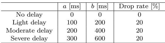
The simulation covers four delay conditions, from a zero-delay, zero-loss baseline to light, moderate, and severe stochastic delay profiles. The three delayed profiles share the same 20 percent drop rate while their delay ranges increase progressively. This setup allows controlled comparison of controller performance as delay severity increases. The zero-delay baseline has 0 ms delay bounds and a 0 percent drop rate. All three non-zero delay profiles share a 20 percent drop rate. Delay bounds are 100 to 200 ms for light delay, 200 to 400 ms for moderate delay, and 300 to 600 ms for severe delay.

In simulation, the proposed controller maintained low position and yaw RMSE across all delay conditions in the stabilization task, while the reference-only controller degraded sharply under moderate and severe delay. In the tracking task, the proposed controller also kept position and yaw errors much lower than the reference-only controller across the reported delay levels, with reference-only yaw error growing dramatically. Severe-delay tracking results were not reported. In stabilization, the proposed controller kept position and yaw RMSE nearly constant across no, light, moderate, and severe delay conditions, whereas the reference-only controller showed large error growth under moderate and severe delay. In tracking, reference-only yaw RMSE was substantially higher than the proposed controller even without delay and increased sharply with delay, while the proposed controller's errors remained relatively low.

The simulation evaluates a proposed controller against a reference-only controller on stabilization and tracking tasks under four delay conditions: a zero-delay, zero-loss baseline and light, moderate, and severe stochastic delay profiles with a shared 20 percent drop rate and increasing delay bounds. The stabilization experiment shows that the proposed controller keeps position and yaw RMSE nearly constant as delay severity increases, while the reference-only controller degrades sharply under moderate and severe delay. The tracking experiment similarly shows the proposed controller maintaining much lower position and yaw errors across reported delay levels, while reference-only yaw error grows substantially even without delay; severe-delay tracking results were not reported.