一句话总结

Snell 和 Griffiths 将保形预测重新表述为贝叶斯求积，提供了一种实用的分布无关不确定性量化方法，用可解释的贝叶斯预测替代频率派保证，以预测高风险机器学习系统在测试时可能损失的区间范围。

核心贡献

• 该论文从贝叶斯视角重构面向黑盒预测器（包括深度神经网络）的分布无关不确定性量化，将保形预测、统计预测分析和贝叶斯求积联系起来。

• 所提方法将贝叶斯求积应用于校准损失，以构建测试时损失的非参数后验，从而提供可解释的保证，并比频率派界限给出更丰富的可能损失范围表示。

• 两种常见频率派方法成为该方法的特例，并且贝叶斯形式使假设更明确，允许纳入额外知识，并减少过于乐观的保证。

引言

深度学习系统越来越多地用于医学和金融等高风险领域，模型不仅需要整体表现良好，还必须满足公平性要求并限制造成危害的概率。这使得评估黑盒预测模型是否适合部署变得尤为重要，尤其是在训练细节不可用或属于专有信息的情况下。

Prior distribution-free methods such as conformal prediction can provide finite-sample performance guarantees, but they are rooted in frequentist statistics. This makes it difficult to incorporate available domain knowledge, such as data distribution assumptions or model-specific constraints, and they often emphasize expected loss across hypothetical datasets rather than the full distribution of outcomes relevant to observed data.

The authors develop a Bayesian framework for uncertainty quantification by modeling uncertainty in quantile values and constructing a nonparametric characterization of possible deployment distributions from a calibration set. This approach connects conformal prediction to statistical prediction analysis and Bayesian quadrature, recovers split conformal prediction and conformal risk control as special cases, and provides a richer, more interpretable view of performance guarantees while still allowing distribution-free analysis.

方法

The authors begin by casting uncertainty calibration as a decision problem. Let $z=(z_1,\ldots,z_n)$z=(z1​,…,zn​) be calibration data, with $z_i=(x_i,y_i)$zi​=(xi​,yi​), and let a future test point follow the same distribution. A control parameter $\lambda$λ, such as a score threshold, is chosen from the calibration data and induces a loss $L(\theta,\lambda)$L(θ,λ) under the unknown state of nature $\theta$θ. The risk of a decision rule is

$$R(\theta,\lambda)=\int L(\theta,\lambda(z))f(z\mid\theta)\,dz,$$R(θ,λ)=∫L(θ,λ(z))f(z∣θ)dz,

and the distribution-free objective is to find a rule whose worst-case risk is controlled:

$$\bar R(\lambda)=\sup_\theta R(\theta,\lambda)\le \alpha.$$Rˉ(λ)=θsup​R(θ,λ)≤α.

Any rule satisfying this condition is called $\alpha$α-acceptable. Split conformal prediction corresponds to choosing $\lambda$λ so that the miscoverage loss remains below the target level. The threshold is obtained from the ordered nonconformity scores:

$$\lambda_{\mathrm{scp}} = \begin{cases} s_{(\lceil (n+1)(1-\alpha)\rceil)}, & \text{if } \lceil (n+1)(1-\alpha)\rceil\le n,\\ \infty, & \text{otherwise}. \end{cases}$$λscp​={s(⌈(n+1)(1−α)⌉)​,∞,​if ⌈(n+1)(1−α)⌉≤n,otherwise.​

Conformal risk control generalizes this idea by allowing a monotonic non-increasing individual loss $\ell(z_{\mathrm{new}},\lambda)$ℓ(znew​,λ) and selecting

$$\lambda_{\mathrm{crc}} = \inf\left\{ \lambda: \frac{1}{n+1} \left( \sum_{i=1}^{n}\ell(z_i,\lambda)+B \right) \le \alpha \right\}.$$λcrc​=inf{λ:n+11​(i=1∑n​ℓ(zi​,λ)+B)≤α}.

The authors then reinterpret these constructions through Bayesian decision theory. Instead of treating $\theta$θ as known while data are unknown, they condition on the observed calibration losses and reason about the posterior distribution of the risk. If the individual losses can be written as an expectation over a loss quantile function $K(t)$K(t), then

$$L(\theta,\lambda) = \int_0^1 K(t)\,dt.$$L(θ,λ)=∫01​K(t)dt.

This suggests a Bayesian quadrature procedure: place a prior over quantile functions, update it using observed loss values, and integrate the expected loss. As shown in the figure below:

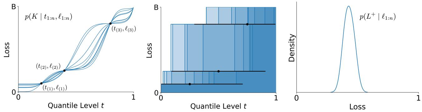
The standard Bayesian quadrature view places a prior over the quantile function and updates it after observing both loss values and their quantile levels. In conformal prediction, however, the quantile levels corresponding to the calibration losses are not directly observed. The authors therefore combine a right rectangular integration rule with distribution-free results on quantile spacings.

To remove the dependence on a prior over quantile functions, they upper-bound the posterior expected loss using only the ordered calibration losses. Let $\ell_{(1)}\le \cdots \le \ell_{(n)}$ℓ(1)​≤⋯≤ℓ(n)​ be the ordered observed losses, and set $\ell_{(n+1)}=B$ℓ(n+1)​=B for a known loss upper bound. The worst-case posterior expectation satisfies

$$\sup_\pi \mathbb{E}(L\mid t_{1:n},\ell_{1:n}) \le \sum_{i=1}^{n+1} u_i \ell_{(i)}, \qquad u_i=t_{(i)}-t_{(i-1)}.$$πsup​E(L∣t1:n​,ℓ1:n​)≤i=1∑n+1​ui​ℓ(i)​,ui​=t(i)​−t(i−1)​.

Thus the problem reduces to assigning weights to the observed ordered losses. The uncertainty over the quantile locations is handled through probability integral transform properties. If losses are i.i.d. with continuous distribution, then the spacings between consecutive ordered quantile levels follow a Dirichlet distribution:

$$(u_1,\ldots,u_{n+1})\sim \mathrm{Dir}(1,\ldots,1).$$(u1​,…,un+1​)∼Dir(1,…,1).

The authors define a random variable

$$L^{+} = \sum_{i=1}^{n+1} U_i \ell_{(i)}, \qquad (U_1,\ldots,U_{n+1})\sim \mathrm{Dir}(1,\ldots,1).$$L+=i=1∑n+1​Ui​ℓ(i)​,(U1​,…,Un+1​)∼Dir(1,…,1).

They show that $L^{+}$L+ stochastically dominates the posterior expected loss under any prior:

$$\inf_\pi \Pr(L\le b\mid \ell_{1:n}) \ge \Pr(L^{+}\le b).$$πinf​Pr(L≤b∣ℓ1:n​)≥Pr(L+≤b).

Therefore, for a target probability $\beta$β, the critical value

$$b_\beta^* = \inf_b \left\{ b: \Pr(L^{+}\le b\mid \ell_{1:n})\ge \beta \right\}$$bβ∗​=binf​{b:Pr(L+≤b∣ℓ1:n​)≥β}

provides a valid upper confidence bound on the risk. The left part of the next figure illustrates why considering only the average expected loss can underestimate the risk, whereas the proposed approach incorporates variability from unknown quantile levels:

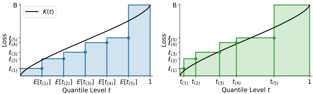
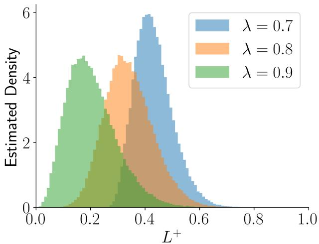
In practice, the distribution of $L^{+}$L+ can be approximated by sampling Dirichlet weights and forming weighted combinations of the ordered losses. This yields a posterior-like distribution over plausible expected losses for each candidate decision parameter $\lambda$λ. The density of $L^{+}$L+ shifts as $\lambda$λ changes, allowing the method to evaluate how conservative the resulting risk bound is for different candidate thresholds:

The existing conformal procedures appear as special cases when only the expectation of $L^{+}$L+ is used. Since

$$\mathbb{E}(L^{+}) = \sum_{i=1}^{n+1}\mathbb{E}(U_i)\ell_{(i)} = \frac{1}{n+1} \left( \sum_{i=1}^{n}\ell_i+B \right),$$E(L+)=i=1∑n+1​E(Ui​)ℓ(i)​=n+11​(i=1∑n​ℓi​+B),

conformal risk control corresponds to selecting the smallest $\lambda$λ satisfying

$$\mathbb{E}(L^{+})\le \alpha.$$E(L+)≤α.

For split conformal prediction, the loss is $\ell_i=1-\mathbb{1}\{s_i\le \lambda\}$ℓi​=1−1{si​≤λ}. If $\lambda=s_{(k)}$λ=s(k)​, then

$$\mathbb{E}(L^{+}) = 1-\frac{k}{n+1},$$E(L+)=1−n+1k​,

so the condition $\mathbb{E}(L^{+})\le \alpha$E(L+)≤α is satisfied whenever

$$k\ge (n+1)(1-\alpha).$$k≥(n+1)(1−α).

Thus the approach preserves the familiar conformal thresholds while extending the analysis from a single expected-loss estimate to the full upper-bounding distribution of possible expected losses.

实验

Experiments on synthetic loss distributions, synthetic heteroskedastic prediction intervals, and MS-COCO multilabel classification evaluate repeated calibration splits by measuring how often the chosen risk threshold is exceeded and how large the resulting prediction sets or intervals become. The synthetic settings validate that the posterior-based highest posterior density rule provides a stronger data-conditional risk guarantee than marginal conformal risk control, reducing excessive-risk trials while still controlling failure rates. On MS-COCO, the proposed method better balances risk control and efficiency than baselines, keeping false-negative-rate risk within the allowed bound while producing shorter prediction sets than more conservative approaches.

Across repeated trials, CRC exceeds the target risk threshold much more often than RCPS or the proposed method. RCPS shows almost no threshold violations, while the proposed method also keeps violations extremely rare and is described as offering shorter prediction intervals than the baselines. Together, these results support a practical balance between empirical risk compliance and prediction efficiency. CRC has the highest frequency of threshold exceedance among the compared decision rules. RCPS controls the risk conservatively, with nearly zero observed violations. The proposed method maintains very low violation frequency while targeting smaller prediction sets or intervals.

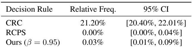
The synthetic heteroskedastic experiment shows a tradeoff between risk-threshold violations and prediction interval length. Split conformal prediction and conformal risk control often exceed the target risk threshold, while producing shorter intervals, whereas RCPS essentially avoids violations but requires much longer intervals. The proposed method with beta = 0.95 keeps violations low while producing intervals shorter than RCPS. The proposed method balances failure-rate control and interval length more effectively than the compared baselines. RCPS is highly conservative in excess-risk violations but incurs a larger interval-length cost. The method achieves low violations without yielding intervals as long as the strictly conservative RCPS baseline.

The results show a tradeoff between risk-threshold exceedance and prediction set size. CRC uses the smallest prediction sets but exceeds the target risk threshold most frequently, while RCPS avoids threshold exceedance in the reported trials but produces the largest prediction sets. The proposed method with beta = 0.95 reduces frequent threshold exceedance relative to CRC while keeping prediction sets smaller than those of RCPS. CRC yields the smallest prediction sets but the highest relative frequency of threshold exceedance. RCPS avoids threshold exceedance in the reported trials but at the cost of larger prediction sets. The proposed method balances risk control and set compactness, exceeding the threshold much less often than CRC while using shorter sets than RCPS.

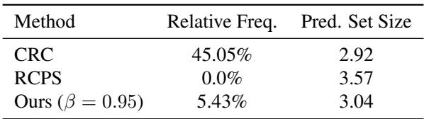
Across repeated synthetic experiments comparing risk-control methods, CRC tends to satisfy thresholds with compact intervals or sets but frequently exceeds the target risk, whereas RCPS is highly conservative and nearly eliminates violations at the cost of substantially larger intervals or sets. The proposed method achieves a more favorable balance by maintaining very low threshold exceedance while producing shorter intervals and smaller prediction sets than RCPS. Overall, these results show that the method provides a practical tradeoff between empirical risk compliance and predictive efficiency.