One-sentence Summary

Researchers at Google Research propose a decoder-only foundation model for time-series forecasting that, through pretraining with input patching on a large corpus of real-world and synthetic data, achieves zero-shot accuracy close to state-of-the-art supervised models across diverse public datasets, demonstrating robust performance across domains, horizons, and temporal granularities.

Key Contributions

• Introduces TimesFM, a decoder-style attention model with input patching, pretrained on a large corpus of real-world and synthetic time-series data (around 100B timepoints) to serve as a general-purpose zero-shot forecaster.
• The model maps any time-series context directly to a forecast horizon without dataset-specific covariates, enabling out-of-the-box predictions across diverse domains, horizons, and temporal granularities.
• Experiments on previously unseen public datasets show that TimesFM’s zero-shot forecasts approach the accuracy of state-of-the-art supervised models for each dataset, while outperforming pretrained LLM-based zero-shot forecasters at a much smaller model size.

Introduction

Time-series forecasting is critical across domains like retail, energy, traffic, and weather, where deep learning models have become the standard approach, often outperforming classical statistical methods such as ARIMA. However, these models are typically trained in a supervised setting for specific datasets, requiring significant data and compute resources for each new forecasting task. Prior work has explored transfer learning or fine-tuning large language models (LLMs) like GPT-3 for forecasting, but these approaches either lack a single pretrained model that generalizes broadly or incur prohibitive costs due to massive model sizes.

The authors address this gap by introducing TimesFM, a foundation model for time-series forecasting that achieves near state-of-the-art zero-shot accuracy on unseen datasets across diverse domains, without any fine-tuning. They overcome key challenges, including the lack of a defined vocabulary in time-series data, varying context and horizon lengths, and limited public time-series data, by building a large-scale corpus from real-world sources like web search queries and Wikipedia page visits, supplemented with synthetic data. Their main contribution is a compact decoder-style attention architecture with input patching, pretrained on this corpus, which delivers superior zero-shot performance compared to LLM-based forecasters at a tiny fraction of the parameter and data scale.

Dataset

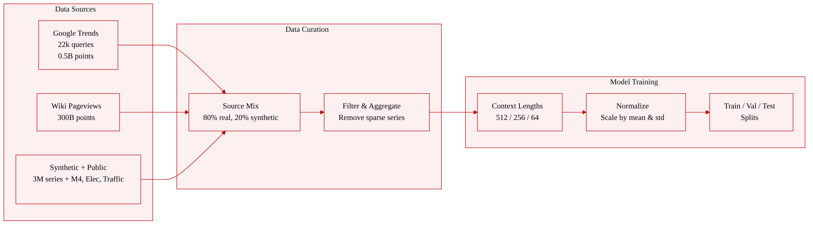
The authors construct a pretraining corpus for a time-series foundation model by combining three major sources: Google Trends, Wiki Pageviews, and synthetic data, supplemented with several public datasets. The goal is to achieve sufficient volume and diversity to cover various domains, trend and seasonality patterns, and time granularities relevant to forecasting use cases.

Dataset composition and sources

• Google Trends: Captures search interest over time for millions of queries. The authors select around 22k "head" queries based on search interest over 15 years (2007 to 2022). Beyond these queries, the time-series become more than 50% sparse. They download search interest at hourly, daily, weekly, and monthly granularities. Date ranges are Jan. 2018 to Dec. 2019 for hourly data and Jan. 2007 to Dec. 2021 for other granularities. This subset amounts to roughly 0.5 billion time-points.
• Wiki Pageviews: Captures hourly views of all Wikimedia pages. The authors download all pageview data from Jan. 2012 to Nov. 2023, clean and aggregate views by page into hourly, daily, weekly, and monthly granularities, and filter out time-series with excessive zeros. The final corpus contains roughly 300 billion time-points.
• Synthetic Data: Generated using ARMA processes, seasonal patterns (mixtures of sines and cosines), trends (linear, exponential with change-points), and step functions. A synthetic time-series can be an additive combination of one or more of these processes. The authors create 3 million synthetic time-series, each of length 2048 time-points.
• Other real-world data sources: The corpus also includes all granularities of the M4 dataset (around 100k time-series), the hourly and 15-minute Electricity and hourly Traffic datasets (with over 300 and over 800 time-series respectively, each having tens of thousands of time-points), the 10-minute granularity Weather dataset, and all 15-minute granularity traffic time-series from a separate source.

Dataset mixing and training usage

• The training loader samples 80% real data and 20% synthetic data.
• The real data mixture gives equal weights to four groups: hourly plus sub-hourly, daily, weekly, and monthly datasets.
• Maximum context length is set to 512 for time-series that are long enough. For weekly granularity, the context length is reduced to 256 because the time-series are not sufficiently long. For monthly granularity, the context length is further reduced to 64.
• The authors apply only the standard normalization part of reversible instance normalization, meaning each time-series context is scaled by the context mean and standard deviation of the first input patch in the context.

Method

The authors introduce TimesFM, a foundation model for time-series forecasting designed to adapt to variable context and horizon lengths. The architecture is built upon several key guiding principles. First, the authors leverage patching, breaking down the time-series into contiguous non-overlapping patches, which act as analogues to tokens in language models and reduce the number of tokens fed into the transformer. Second, the model is trained in a decoder-only mode, optimizing the prediction of the next patch as a function of all past patches in parallel over the entire context window. Third, to balance accuracy and efficiency, the authors introduce longer output patches, allowing the model to predict a larger chunk of the time-series based on encoded input patches rather than generating one token at a time. Finally, patch masking is employed during training to ensure the model can handle all possible context lengths.

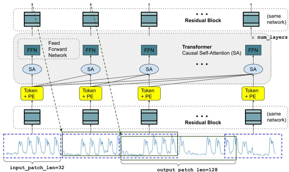
The model architecture consists of three main components: input layers, stacked transformer layers, and output layers. The input layers preprocess the time-series into input tokens. The input sequence $\mathbf{y}_{1:L}$y1:L​ is divided into patches of size $p$p. A binary padding mask $\mathbf{m}_{1:L}$m1:L​ is applied to ignore specific inputs. Each patch $\tilde{\mathbf{y}}_j$y~​j​ is processed by a Residual Block, which is a Multi-layer Perceptron with a skip connection, and combined with positional encoding $\mathrm{PE}_j$PEj​ to form the $j$j-th input token:

where $\tilde{\mathbf{m}}_j$m~j​ is the patched mask.

The core of the model comprises $n_l$nl​ stacked transformer layers. Each layer features multi-head causal self-attention followed by a feed-forward network. Causal attention ensures that each output token can only attend to preceding input tokens. The output of the transformer for the $j$j-th token is computed as:

where $\dot{m}_j$m˙j​ indicates whether the patch is masked.

The output layers map the transformer output tokens to predictions. Unlike standard language models, the output patch length $h$h can be larger than the input patch length $p$p. A second Residual Block maps the output token $\mathbf{o}_j$oj​ to predict the subsequent $h$h time-points:

For training, the authors focus on point forecasting and minimize the Mean Squared Error loss across all patches in a mini-batch:

To enable the model to handle varying context lengths, a specific random masking strategy is used. For each time-series, a random number $r$r between 0 and $p-1$p−1 is sampled, and the first $r$r time-points of the first input patch are masked. This allows the model to effectively learn from all context lengths from 1 to the maximum training context length.

During inference, the trained network produces forecasts for any horizon using auto-regressive decoding. Given an input sequence, the model predicts the next output patch. This prediction is then concatenated with the original input and fed back into the network to generate the subsequent output patch, repeating the process until the desired horizon is reached. If the input length is not a multiple of the patch size, zeros are appended and masked accordingly.

Experiment

The model is evaluated in zero-shot settings across Monash, Darts, and Informer datasets, where it matches or outperforms supervised baselines, including state-of-the-art methods like PatchTST, despite never being trained on these benchmarks. Ablation studies confirm that scaling model size and FLOPs monotonically reduces error, longer output patch lengths improve autoregressive decoding for long horizons, and an input patch length of 16 or 32 yields the best trade-off between performance and training speed. Adding synthetic data is shown to be critical for generalizing to underrepresented granularities, as it significantly boosts performance on datasets with unusual frequencies like 15-minute intervals, while having minimal impact on well-represented hourly data.

The pretraining dataset combines synthetic and real-world time series across various granularities, with synthetic data contributing the largest volume. The design choices around patch lengths and dataset composition are validated by experiments showing performance trade-offs. Synthetic data dominates the pretraining mix, providing billions of time points to supplement real datasets. Real datasets span hourly, daily, 10-minute, and 15-minute granularities, covering domains like electricity, traffic, weather, sales, and urban mobility. Increasing output patch length reduces forecasting error monotonically for long-horizon tasks. Input patch length shows an optimal range around 16-32, balancing accuracy and training efficiency. Removing synthetic data hurts performance on underrepresented granularities, especially 15-minute data, while hourly data is less affected.

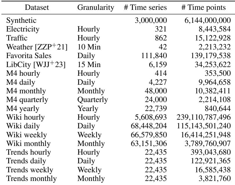
The pretraining dataset mixes synthetic and real-world time series across multiple granularities, with synthetic data providing the largest volume. Experiments validate that an output patch length increase monotonically reduces forecasting error for long horizons, while an input patch length around 16-32 balances accuracy and training efficiency. Removing synthetic data significantly degrades performance on underrepresented granularities, particularly 15-minute data, whereas hourly data remains relatively robust.