One-sentence Summary

Stability AI scales rectified flow transformers for high-resolution text-to-image synthesis by introducing perceptually-biased noise sampling and a novel transformer architecture with separate image and text token weights that enables bidirectional cross-modal attention, demonstrating predictable scaling trends and state-of-the-art performance across automated metrics and human evaluations.

Key Contributions

• Introduces a reweighted timestep sampling method for training rectified flow models that biases timestep selection toward perceptually relevant scales, and a large-scale study shows improved high-resolution text-to-image synthesis over established diffusion formulations while retaining few-step sampling advantages.
• Presents a transformer-based multimodal architecture for text-to-image generation that uses separate image and text token streams with modality-specific weights and bidirectional information flow, improving text comprehension, typography, and human preference ratings over UViT and DiT backbones.
• Conducts a scaling study up to 8 billion parameters and 5 x 10^22 FLOPs, demonstrates predictable scaling trends, and shows that lower validation loss correlates with stronger results on T2I-CompBench, GenEval, and human evaluations. The largest models outperform SDXL, SDXL-Turbo, Pixart-α, and DALL-E 3.

Introduction

Diffusion models generate images and videos by reversing noise, and they have become a leading approach for high resolution text to image synthesis. This matters because these models can produce diverse, high quality media, but their iterative sampling can be slow and expensive, making more efficient formulations important.

Prior work faces two main limitations. First, the choice of forward path from data to noise affects both generation quality and sampling efficiency; straight-line rectified flow has appealing properties, but it had not been widely proven in large scale text-to-image settings. Second, common architectures often feed a fixed text representation into the image model through one-way mechanisms such as cross-attention, which can limit how text and image information interact during generation.

The authors address these gaps by introducing improved noise weighting and samplers for rectified flow models, and by proposing a multimodal transformer architecture with separate image and text token streams that allows bidirectional information flow. They then scale this combination up to an 8B parameter model with 5 x 10^22 training FLOPs, showing that lower validation loss tracks closely with better benchmark and human evaluations, and that their approach outperforms prior open and closed systems.

Dataset

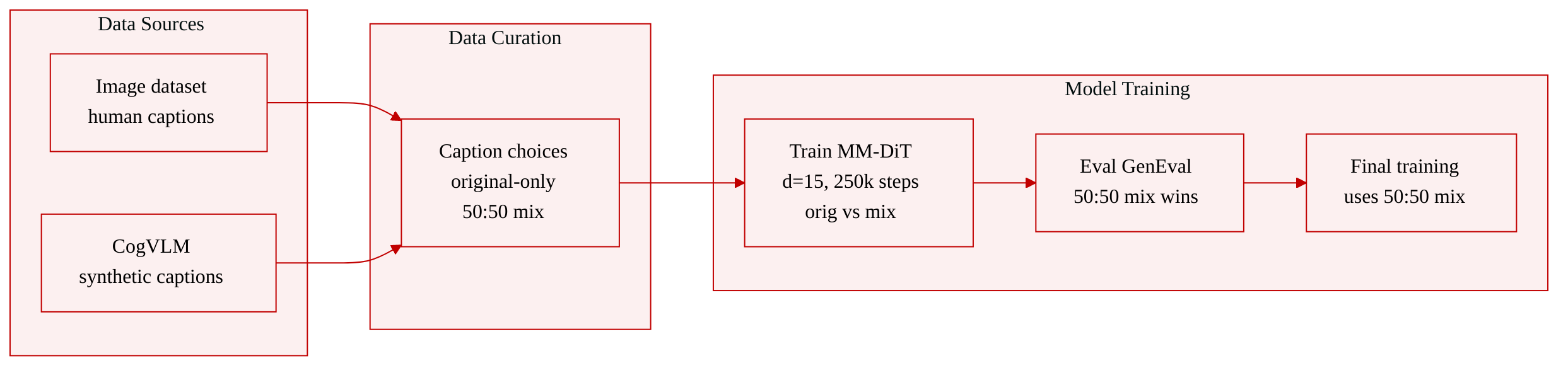
• The authors use a large-scale image dataset with existing human-written captions as the base data source.

• To improve caption quality, they generate synthetic captions with the off-the-shelf vision-language model CogVLM.

• They mix original captions and synthetic captions in a 50:50 ratio to preserve concepts that may be missing from synthetic-only captions.

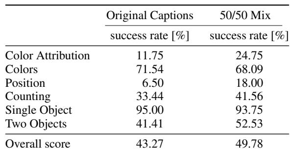
• They compare original-only captions and the 50:50 caption mix by training two d=15 MM-DiT models for 250k steps and evaluating them on GenEval.

• The experiments show that the 50:50 original and synthetic caption mixture performs better, so this mixed-caption format is used for the rest of the model training.

Method

The authors leverage a simulation-free flow-matching formulation to train a conditional generative model without differentiable ODE solving during training. The model is defined through a time-dependent velocity field $v_\Theta(y_t,t)$vΘ​(yt​,t) that parameterizes an ODE

Instead of integrating this ODE to obtain training targets, the authors construct a forward probability path between the data distribution $p_0$p0​ and a Gaussian noise distribution $p_1 = \mathcal{N}(0,1)$p1​=N(0,1). For a clean sample $x_0$x0​ and Gaussian noise $\epsilon$ϵ, the interpolated latent state is

with boundary choices $a_0=1$a0​=1, $b_0=0$b0​=0, $a_1=0$a1​=0, and $b_1=1$b1​=1, so that $z_0$z0​ follows $p_0$p0​ and $z_1$z1​ follows $p_1$p1​. The conditional transport map is

and its induced conditional vector field is

The marginal vector field that generates the marginal probability path $p_t(z_t)$pt​(zt​) would require expectation over $\epsilon$ϵ, which is intractable in general. The method therefore optimizes a Conditional Flow Matching objective using conditional targets:

This objective has the same minimizer as the intractable marginal objective but remains tractable because $u_t(z|\epsilon)$ut​(z∣ϵ) can be computed explicitly. For the linear interpolation class above, the conditional target can be rewritten as

Introducing the log signal-to-noise ratio

the target becomes

This reparameterization allows the flow objective to be expressed as a weighted noise-prediction loss. By defining

the training objective can be written in a unified weighted form

The original Conditional Flow Matching loss corresponds to the weighting

The choice of trajectory $z_t$zt​ determines the weighting $w_t$wt​ and the type of network prediction used during training. The method considers several probability paths. Rectified Flow defines straight-line interpolation

which yields the weighting

and directly parameterizes velocity. EDM uses a variance-exploding style path

with a log-normal noise distribution induced by the chosen scale schedule and a prediction target related to F-prediction. A cosine schedule defines

and can be paired with either $\epsilon$ϵ-prediction or $v$v-prediction, giving different time-dependent weights. Latent diffusion variants also use variance-preserving schedules where $b_t=\sqrt{1-a_t^2}$bt​=1−at2​​ and $a_t$at​ is constructed from a discrete diffusion coefficient sequence $\beta_t$βt​, with different linearized or scaled schedules for $\beta_t$βt​.

Beyond choosing the trajectory, the authors tailor the distribution from which training timesteps are sampled. For Rectified Flow, uniform timestep sampling is equivalent to training velocity uniformly across all times. However, the prediction target $\epsilon-x_0$ϵ−x0​ is often hardest in the middle of the trajectory, because the conditional mean changes rapidly around intermediate noise levels. Sampling $t$t from a non-uniform density $\pi(t)$π(t) is equivalent to using a weighted loss with

One proposed density is the logit-normal distribution

where

In practice, a sample is generated by drawing $u\sim\mathcal{N}(m,s)$u∼N(m,s) and mapping it through the logistic function. The location parameter $m$m biases training toward either data-like or noise-like regions, while the scale parameter $s$s controls concentration around the chosen timestep region.

Because the logit-normal density vanishes at the endpoints, the authors also use a mode-sampling distribution with heavy tails. For a scale parameter $s$s, define

For a valid monotonic range of $s$s, this defines an invertible mapping, and the induced timestep density is

Positive values of $s$s emphasize the middle of the trajectory, negative values emphasize endpoints, and $s=0$s=0 recovers uniform sampling. Another variant, CosMap, constructs a time map from a uniform variable $u$u so that the log-SNR matches the cosine schedule. It uses

with density

For text-conditional generation, the model operates in the latent space of a pretrained autoencoder. An input RGB image $X\in\mathbb{R}^{H\times W\times 3}$X∈RH×W×3 is mapped by an encoder $E$E into a lower-dimensional latent representation

Reconstruction quality of this autoencoder constrains the maximum achievable generated image quality, and the architecture chooses a latent width $d=16$d=16 as a design point that balances reconstruction fidelity with diffusion-model learning capacity. Text conditioning is produced by frozen pretrained text encoders. The method combines coarse pooled text information with fine-grained token sequences. A pooled text vector $c_{\mathrm{vec}}$cvec​ is used for global modulation, while a sequence representation $c_{\mathrm{ctxt}}$cctxt​ is supplied to the transformer backbone so that detailed phrase and word-level information is accessible during generation. Refer to the architecture overview:

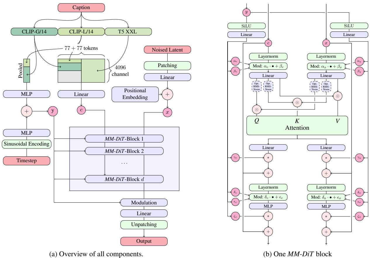
The diffusion backbone is a multimodal transformer that operates on a sequence of latent image patches and text tokens. The noised latent is first patchified by flattening $2\times2$2×2 patches, producing a sequence of length

This patch sequence and the text-token sequence are embedded into a common dimensionality and concatenated. Each block contains modulated attention and MLP operations. For each modality, layer normalization is followed by a modulation path driven by the global conditioning vector. Conceptually, for modality $m\in\{c,x\}$m∈{c,x}, the pre-attention state can be written as

where $\alpha_m$αm​ and $\beta_m$βm​ are predicted from the conditioning vector. The text and image streams then produce modality-specific query, key, and value projections. These projections are concatenated so that attention is computed over the joint token sequence. This allows image tokens and text tokens to interact, while preserving separate learned transformations for each modality. Optional RMS normalization on queries and keys can be used to stabilize training. After attention, a residual branch applies a predicted scaling factor

The MLP sublayer uses the same pattern, with additional modulation and scaling parameters for the feed-forward transformation. The network uses two sets of trainable parameters, one for the text stream and one for the image stream, while sharing the attention computation. This is equivalent to having two modality-specific transformer pathways that exchange information through joint attention, rather than using cross-attention from one fixed token sequence to another. The model is parameterized in terms of depth $d$d, with hidden size $64d$64d, MLP width $4\cdot64d$4⋅64d, and number of attention heads equal to $d$d.

During training, a clean latent sample and its text conditioning are encoded, a timestep is sampled from the selected density, noise is added according to the chosen forward process, and the network predicts either velocity, noise, or an equivalent target depending on the parameterization. The loss is a weighted prediction error evaluated on the concatenated text-image token sequence. During inference, noise is sampled from $p_1$p1​, the learned ODE is integrated forward in time to produce a latent sample, and the autoencoder decoder maps the latent back to image space.

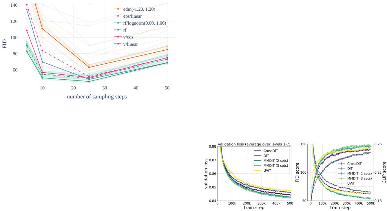
When compared against transformer diffusion backbones under the same training setup, the two-weight multimodal backbone shows more favorable optimization than baseline architectures that use shared weights, cross-attention, or convolutional hybrid designs. The comparison also shows that increasing the number of separate parameter sets beyond two gives only a small gain relative to its additional parameter and memory cost. As shown in the figure below:

Experiment

Experiments evaluate training formulations for rectified flows under controlled comparisons on ImageNet and CC12M, then assess model components for text-to-image synthesis. The training comparison validates that nonuniform timestep sampling, especially a lognormal schedule emphasizing intermediate timesteps, improves robustness across metrics and sampler settings, while modified rectified-flow formulations can outperform established diffusion losses. Component studies further show that a higher-capacity latent autoencoder, mixed synthetic and original captions, and the proposed MM-DiT backbone each enhance generation quality and prompt fidelity. Finally, scaling to large image and video models shows steady validation-loss improvements with size and compute, with larger models achieving stronger benchmark and human-preference results while requiring fewer sampling steps.

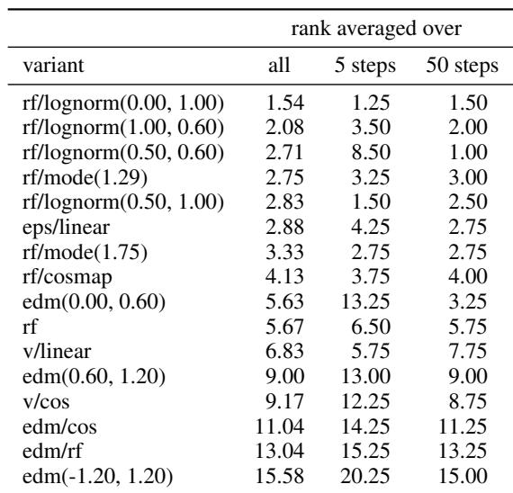
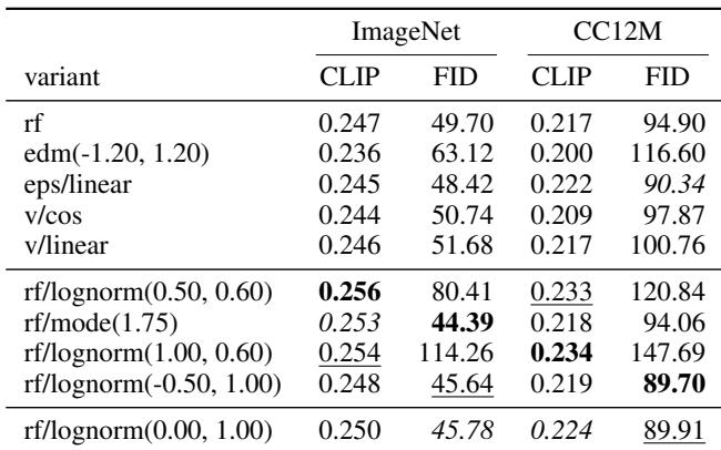
Across the tested formulations, rectified-flow variants with lognormal timestep weighting place at or near the top of the global ranking when performance is averaged over weight types, datasets, and sampling settings. These variants remain broadly competitive, while individual settings show different strengths in fewer-step and many-step evaluations. The conventional epsilon prediction with a linear schedule is also strong but trails the leading lognormal variants overall. Lognormal RF weighting is consistently among the strongest overall variants. Some lognormal settings rank very well at 5 steps but differ at 50 steps. The mode-based RF variant is competitive but slightly behind the best lognormal variants. Epsilon prediction with a linear schedule remains a strong baseline.

Across the compared variants at 25 sampling steps, the rf/lognorm(0.50, 0.60) setting gives the strongest CLIP scores on both datasets, while edm(-1.20, 1.20) gives the best FID scores. This points to a tradeoff between text alignment and image fidelity. The other variants fall between these extremes, with v/cos performing especially well on FID among the v-prediction variants. rf/lognorm(0.50, 0.60) reaches the highest CLIP scores, indicating stronger alignment with text prompts. edm(-1.20, 1.20) obtains the lowest FID scores and remains competitive on CLIP, suggesting a strong balance of fidelity and alignment.

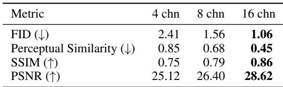
Increasing the number of latent channels from 4 to 16 while keeping the downsampling factor fixed at 8 consistently improves autoencoder reconstruction. The higher channel configurations show lower FID and perceptual similarity, along with higher SSIM and PSNR. This indicates that wider latent spaces provide a stronger reconstruction ceiling for latent diffusion models. More latent channels improve reconstruction quality across the reported metrics. The 16 channel configuration gives the best overall fidelity and similarity.

A 50/50 mix of synthetic and original captions improves text-to-image performance on GenEval compared with training on original captions only. The improvement is most visible in compositional tasks that require spatial placement, counting, attribute assignment, and two-object scenes, while simple object and color evaluations remain broadly high. Synthetic captions trained with original captions improve overall text-to-image prompt compliance. The mixed-caption setting gains most on harder compositional and spatial prompt categories. Original captions still perform strongly on simple object and color tasks.

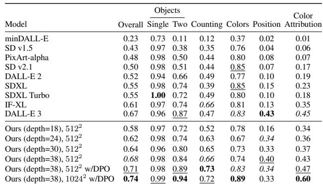
Across GenEval, the largest trained model is reported to achieve the strongest overall prompt-comprehension performance, surpassing current open models and DALLE-3. The comparison shows that single-object generation is relatively strong across models, while counting, spatial placement, and attribute binding remain harder and tend to score lower. Scaling with improved methods and higher training resolution gives the biggest model the best overall result and strong performance in most categories. The largest model is reported to outperform current open models and DALLE-3 on overall GenEval performance Single-object generation is generally the strongest category across the compared models Counting, position, and color attribute binding remain challenging for many models

Experiments evaluate different timestep-weighted prediction formulations, latent capacity, caption mixing, and model scaling for diffusion-based image generation. Lognormal rectified-flow variants are overall strongest, while linear epsilon schedules remain competitive, and comparisons at fixed sampling steps reveal a tradeoff between text alignment and image fidelity. Wider latent spaces consistently improve reconstruction quality, and mixing synthetic captions with original captions enhances prompt compliance, especially on compositional and spatial tasks. Scaling to the largest trained model with higher resolution gives the best overall prompt comprehension, though counting, spatial placement, and attribute binding remain challenging.