One-sentence Summary

Princeton University, UC Berkeley, and Virginia Tech propose In-Run Data Shapley, a method that computes Shapley values at each gradient update iteration and accumulates them throughout a single training run, eliminating the need for model retraining with negligible runtime overhead to enable data attribution at foundation model pretraining scale, with case studies offering insights into copyright implications for generative AI and pretraining data curation.

Key Contributions

• The paper introduces In-Run Data Shapley, which computes Shapley values at each gradient update iteration and accumulates them across a specific training run, removing the need to retrain models on many data subsets.
• Efficient ghost-family computation techniques scale In-Run Data Shapley to foundation model pretraining, and the most optimized implementation adds negligible runtime overhead compared to standard model training.
• Experiments and case studies demonstrate attribution of pretraining data contribution, yielding insights relevant to copyright in generative AI and pretraining data curation.

Introduction

• The authors focus on data attribution for large language models and other foundation models, where knowing each training source’s influence matters for fair compensation, copyright analysis, regulatory risk, and filtering low-quality or harmful data.

• Existing Shapley value frameworks offer a theoretically fair basis for attribution, but prior methods usually require repeated retraining, are computationally infeasible at foundation model scale, and score data for a general training algorithm rather than the actual model being trained.

• The authors introduce In-Run Data Shapley, which estimates Shapley contributions during training by approximating one-step model changes with Taylor expansions and computing the needed gradient dot products or gradient-Hessian-gradient interactions efficiently, making attribution possible for models such as GPT-2 and Pythia-410M.

Dataset

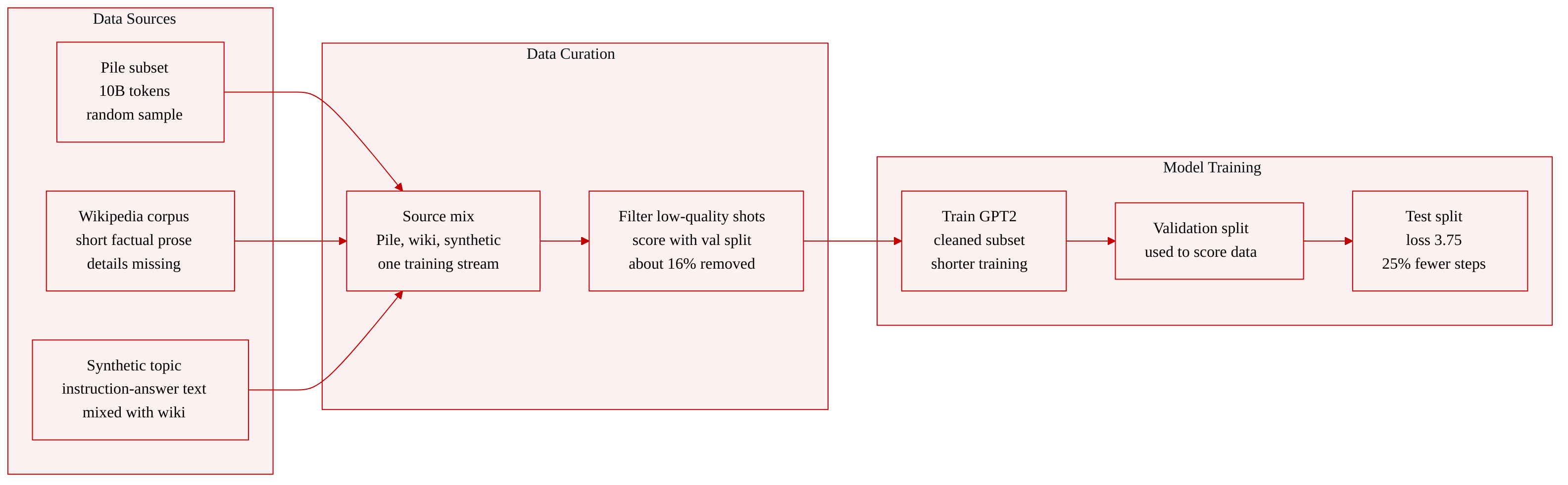
• The authors use a Pile subset as the main training corpus in the case study. They uniformly sample about 10B tokens from the Pile, train a GPT2 model on that subset, and score training points against the Pile validation set. They then remove all negatively valued corpora and retrain on the cleaned subset. The cleaned data reaches a test loss of 3.75 with about 25% fewer training iterations, and about 16% of the subset receives negative second order attribution values. This processing treats attribution scores as a filtering signal for low quality or harmful training examples.

• The authors also reference an Original Wikipedia corpus. It appears to contain short factual or encyclopedic prose passages, with the provided example being a biographical or historical snippet. The excerpt does not report the corpus size, exact filtering rules, schema, training split, or mixture ratio.

• The authors include a Synthetic "Similar topic" corpus nested under the Original Wikipedia corpus. It contains topic-aligned synthetic text, including an instruction-answer style passage and short related domain snippets. The excerpt does not specify its total size, filtering process, metadata fields, or how it is mixed into training.

• The excerpt does not describe a cropping strategy, metadata construction, or formal dataset split for the non-Pile corpora. Quantitative usage details, including scale, filtering, and retraining effects, are provided only for the Pile experiment.

Method

The authors introduce a data attribution framework called In-Run Data Shapley. The central design principle is to avoid retraining the model on exponentially many subsets of the training data. Instead, the method treats a single training run as a sequence of gradient update steps and attributes the loss change at each step to the data points that participated in that step. This creates a “divide and conquer” framework: the original high-level problem of valuing a training set over the full training process is decomposed into many small local attribution problems, one for each mini-batch update. The final score for a data point is the sum of its contributions over all iterations in which it is sampled.

The core idea begins with the usual stochastic training setup. A deep learning model with parameters $w_t$wt​ is trained on a dataset $\mathcal{D}_{\mathrm{tr}} = \{z_i\}_{i=1}^N$Dtr​={zi​}i=1N​ by minimizing a training loss such as $\sum_i \ell(w, z_i)$∑i​ℓ(w,zi​). At iteration $t$t, a mini-batch $\mathcal{B}_t \subseteq \mathcal{D}_{\mathrm{tr}}$Bt​⊆Dtr​ is sampled, and the parameters are updated by

where $\eta_t$ηt​ is the learning rate. A full training run therefore produces a sequence of checkpoints $\{w_0, w_1, \ldots, w_T\}${w0​,w1​,…,wT​}.

To measure the effect of a subset $S$S on a single update, the authors define a local utility function. For a validation point $z^{(\mathrm{val})}$z(val), the utility at iteration $t$t is the counterfactual change in validation loss if only $S$S were used for the gradient update, instead of the full batch $\mathcal{B}_t$Bt​:

where

This local utility is defined over the batch $\mathcal{B}_t$Bt​. It can be extended to the full training set by giving zero influence to points outside $\mathcal{B}_t$Bt​. The resulting per-iteration Shapley value captures only the immediate contribution of each sampled point to that gradient update. Because the batch sampling process is fixed during the training run, the utility function becomes deterministic for that iteration and can also encode other forms of training randomness, such as dropout, by conditioning on the realized state.

The method then aggregates these local utilities across the entire training run. The global utility function is defined as

This represents the cumulative validation-loss change caused by using the subset $S$S across all updates, under the counterfactual assumption that the model follows the same checkpoint trajectory and batch realizations. Since Shapley values are linear with respect to the utility function, the global attribution is simply the sum of the local attributions:

Thus, the final In-Run Data Shapley score for a training point is its cumulative contribution across all gradient updates in which it appears. If the model is evaluated on a validation set $\mathcal{D}^{(\mathrm{val})}$D(val) rather than a single validation point, the authors leverage the same linearity property and compute the total attribution by summing the scores over all validation points.

A key part of the method is making the Shapley calculation tractable. Directly evaluating $U^{(t)}(S)$U(t)(S) for all subsets of a mini-batch is infeasible. The authors therefore approximate the local utility with Taylor expansions around the current model parameters $w_t$wt​. The first-order approximation is

Substituting the gradient update form gives

This approximation is additive over the subset $S$S, so it admits a closed-form Shapley value:

Accumulating over the training run yields the first-order In-Run Data Shapley estimator:

In this formulation, a data point receives positive attribution when its gradient direction at the current checkpoint aligns with the gradient direction of the validation point. A negative attribution indicates that the training point pushed the model in a direction that increased the validation loss. This first-order score is closely related to gradient alignment attribution, but the In-Run Data Shapley perspective clarifies it as the Shapley value of a first-order approximated utility.

The method also includes a second-order approximation. The Taylor expansion of the local utility contains a curvature term involving the Hessian of the validation loss at $w_t$wt​:

The second-order local utility is written as

With the second-order approximation $U^{(t)} \approx U_{(1)}^{(t)} + \frac{1}{2} U_{(2)}^{(t)}$U(t)≈U(1)(t)​+21​U(2)(t)​, the Shapley value still has a closed-form structure. The score for a training point $z$z contains two main components:

The interaction term can be expanded as

This term captures how the presence of other training points in the same batch affects the attributed value of $z$z. Intuitively, if the batch contains many similar or duplicate points, the interaction term redistributes value among them, preventing a single redundant copy from receiving an outsized contribution. As a result, the second-order method measures both the usefulness of a data point with respect to the validation target and its uniqueness within the batch.

The efficient computation module is central to making the method practical. A direct implementation of the first-order estimator would require computing individual gradients for each data point in the batch, which cannot easily exploit ordinary mini-batch GPU training. The authors address this with a “ghost dot-product” technique. The name reflects that individual gradient vectors are never explicitly materialized. Instead, the method reuses quantities already produced during backpropagation.

For a linear layer, the output can be written as

where $\mathbf{W}$W is the weight matrix, $\mathbf{a}$a is the mini-batch input, and $\mathbf{s}$s is the pre-activation output. For sample $i$i, the gradient of its loss with respect to $\mathbf{W}$W can be expressed as an outer product between its input activation and its output gradient:

To compute the dot product between gradients of two samples, the dot product over the outer-product structure can be decomposed into dot products of the smaller activation and output-gradient tensors. For two samples,

Both $\mathbf{a}^{(i)}$a(i) and $\partial \ell^{(i)} / \partial \mathbf{s}^{(i)}$∂ℓ(i)/∂s(i) are already available during backpropagation. Therefore, the pairwise gradient dot products needed for the first-order attribution can be computed within the same backward pass used for the training batch. To include the validation point, the backward pass can be performed on the combined loss

which avoids a separate backward pass solely for the validation point. This design is the main reason the first-order In-Run Data Shapley method can run with minimal extra time beyond standard training.

For the second-order estimator, the challenge is larger because the interaction term requires gradient-Hessian-gradient products. The authors develop a related “ghost” computation that obtains these products with one extra backpropagation per iteration. Rather than forming full gradient-sized vectors for every sample or every data point, the technique exploits the layered structure of neural network gradients and reuses intermediate activations and output gradients. As a result, the second-order method requires approximately two backpropagations per training iteration: one for the combined training and validation computation, and one additional pass for the second-order interaction terms. This is still far cheaper than directly constructing all per-sample gradients and full second-order curvature quantities.

The overall training workflow can be viewed as a standard deep learning loop augmented with attribution bookkeeping. At each iteration, the system samples a batch, performs the usual forward pass, records or reuses the activation and output-gradient information needed for attribution, computes the local first-order contribution terms, optionally computes second-order interaction terms, accumulates per-point scores, and applies the regular parameter update. After training ends, the accumulated per-point scores form the In-Run Data Shapley attribution for the specific model checkpoint produced by that training run.

Experiment

The experiments evaluate In-Run Data Shapley in terms of runtime efficiency, approximation fidelity, and practical data attribution during language model pretraining. They show that the method is computationally feasible, accurately approximates Shapley values, and can identify negatively contributing training data whose removal improves convergence compared with influence-function-based filtering. Additional case studies demonstrate that data values change across training stages and that relevant training corpora can be detected even when outputs are heavily paraphrased, indicating that model behavior can be influenced without verbatim memorization.

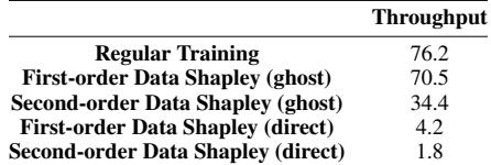
The runtime evaluation shows that first order In Run Data Shapley using ghost dot product throughput is close to regular training throughput. Second order ghost computations are about two times slower than regular training because of extra backpropagation, but both ghost variants are much faster than direct per sample gradient implementations. These efficiency trends make first order and second order In Run Data Shapley more practical than naive approaches. Ghost dot product keeps first order Data Shapley throughput near regular training throughput. Ghost vector Hessian vector product yields second order Data Shapley throughput around half of regular training. Direct implementations have much lower throughput than ghost implementations for both first order and second order computations.

The experiment compares how ranking-based attribution scores the original corpus when validation data varies from paraphrases to topical rewrites. In-Run Data Shapley and the influence function keep the original corpus very high for closely related or semantically similar cases, while BM25 becomes much weaker once lexical overlap disappears. The influence function gives slightly less favorable ranks than In-Run Data Shapley, consistent with noisier leave-one-out estimation. Semantic attribution can surface the original corpus for rewritten or topically related data BM25 tracks verbatim similarity more than broader contribution relevance In-Run Data Shapley ranks the original corpus higher than the influence function in paraphrase cases

The experiments evaluate both the runtime efficiency and ranking behavior of In-Run Data Shapley against influence functions and BM25. They show that ghost-based computations make first-order and second-order attribution substantially more practical than direct per-sample implementations, with ghost methods maintaining throughput close to regular training. The ranking tests further show that semantic attribution methods can identify the original corpus under paraphrased or topically rewritten validation data, whereas BM25 relies too heavily on lexical overlap and becomes much weaker when such overlap disappears.