One-sentence Summary

SSD, a single-shot object detector from researchers at UNC Chapel Hill, Zoox, and Google, discretizes bounding box outputs into default boxes across multiple aspect ratios, scales, and feature map resolutions, completely eliminating proposal generation to achieve 74.3% mAP on VOC2007 at 59 FPS with a $300 \times 300$300×300 input, competitive with Faster R-CNN while being substantially faster.

Key Contributions

• SSD detects objects using a single deep neural network that predicts category scores and bounding-box adjustments for many default boxes at each feature map location, eliminating proposal generation and resampling stages.

• The method attaches convolutional bounding-box predictors to multiple feature maps at different resolutions and samples many locations, scales, and aspect ratios, improving modeling of objects at multiple sizes while remaining simpler than two-stage proposal pipelines.

• Experiments on PASCAL VOC, COCO, and ILSVRC show competitive or better accuracy, with SSD300 reaching 74.3% mAP on VOC2007 at 59 FPS and SSD512 reaching 76.9% mAP, outperforming a comparable Faster R-CNN model.

Introduction

The authors consider modern object detection systems that hypothesize boxes, resample pixels or features, and classify each region, which has enabled high accuracy on benchmarks such as PASCAL VOC and COCO but makes embedded and real-time deployment difficult because of high compute and latency. Prior work reduced speed by optimizing proposals or pooling, yet such gains often traded off detection accuracy, and two-stage region-proposal methods added training and integration complexity. The authors leverage SSD, a single-shot detector that uses fixed default boxes and small convolutional filters to predict object categories and box offsets directly from multiple feature maps and aspect ratio-specific filters, achieving high accuracy without pixel or feature resampling, with real-time performance such as 59 FPS and 74.3% mAP on VOC2007.

Method

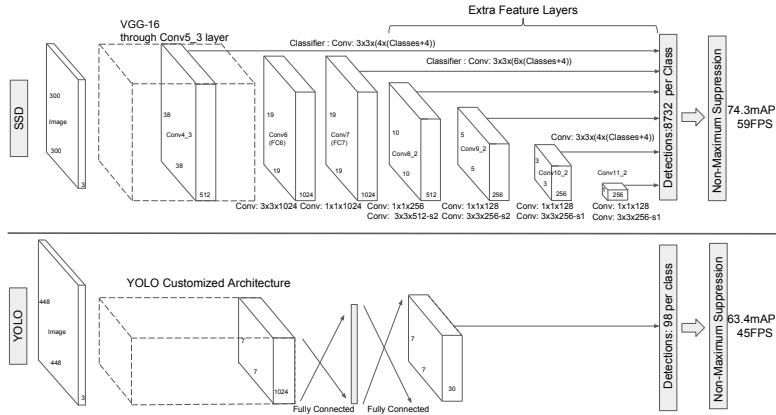
The authors leverage a feed forward convolutional detector that predicts a fixed collection of bounding boxes and class scores in one pass, followed by a non maximum suppression step to obtain final detections. The early layers form a base network, which is a standard classification backbone truncated before the classification layers. Extra feature layers are appended to the end of the base network. These layers progressively reduce spatial resolution, forming multi scale feature maps that allow the model to predict detections for objects of different sizes.

Each feature map, either an existing base network feature map or an added auxiliary feature map, is processed by convolutional predictors. For a feature map of size $m \times n$m×n with $p$p channels, a small $3 \times 3 \times p$3×3×p kernel is applied at each spatial location. For each of the $k$k default boxes associated with that location, the kernel outputs four coordinate offsets and $c$c class confidence values, where $c$c is the number of object classes. This yields $(c+4)k$(c+4)k filters at each location and $(c+4)kmn$(c+4)kmn outputs for the full feature map. The predictors are convolutional rather than fully connected, which allows detection to remain spatially aligned with the feature map. As shown in the framework diagram below:

The central prediction unit is the default box, which is the SSD analogue of an anchor box. Default boxes are assigned to every feature map cell in a convolutional manner, so the relative position of each default box within its cell is fixed. Multiple default boxes per location provide different scales and aspect ratios. At each location, the network predicts offsets from the default box geometry and confidence scores for each class. The offset outputs are not absolute box coordinates; they are corrections relative to the corresponding default box.

The default box tiling, scale variation, and positive or negative assignment during training are shown in the figure below:

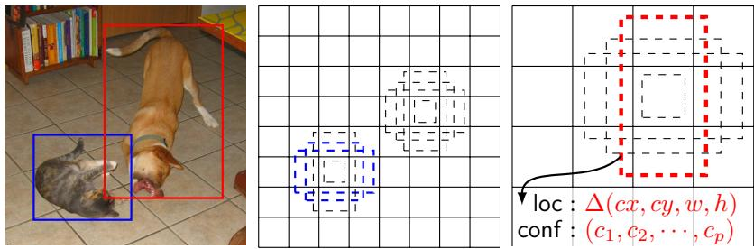
For a default box at a given feature map location with size $|f_k|$∣fk​∣, its center is placed at

This construction lets the network discretize the space of possible object boxes by combining several feature maps, several locations, several scales, and several aspect ratios.

During training, ground truth boxes must be assigned to specific outputs in the fixed set of detector predictions. For each ground truth box, the authors first select the default box with the best Jaccard overlap. They then additionally match any default box whose Jaccard overlap with the ground truth box is above $0.5$0.5. This produces multiple positive matches for some ground truth boxes and simplifies learning by allowing overlapping high quality boxes to receive high scores. The remaining unmatched boxes are treated as negative examples.

The training objective is a weighted sum of a localization loss and a confidence loss. Let $x_{ij}^{p} \in \{1,0\}$xijp​∈{1,0} indicate whether the $i$ith default box is matched to the $j$jth ground truth box of class $p$p. Because multiple default boxes can match one ground truth box, $\sum_i x_{ij}^{p} \geq 1$∑i​xijp​≥1 is possible. The overall loss is

where $N$N is the number of matched default boxes and $\alpha$α is set to $1$1 by cross validation. If $N=0$N=0, the loss is set to $0$0.

The localization loss is a Smooth L1 loss between predicted and ground truth box parameters. The network regresses offsets relative to the default box center, width, and height:

The confidence loss is a softmax loss over multiple classes. Positive default boxes contribute class losses for their matched categories, while negative default boxes contribute background loss:

with

The scale assigned to each feature map is chosen systematically rather than relying on multiple image scales. If $m$m feature maps are used for prediction, the scale for feature map $k$k is computed as

with $s_{\min}=0.2$smin​=0.2 and $s_{\max}=0.9$smax​=0.9. This makes the lowest feature map responsible for smaller objects and the highest feature map responsible for larger objects. The default box width and height for a given aspect ratio $a_r$ar​ are

The authors use aspect ratios $\{1,2,3,\frac{1}{2},\frac{1}{3}\}${1,2,3,21​,31​}. For aspect ratio $1$1, they also add one extra box with scale

which improves coverage between adjacent feature map scales.

After matching, most default boxes are negatives, which creates a severe positive and negative imbalance. To avoid unstable optimization, the authors apply hard negative mining. They rank negative examples by confidence loss and keep only the hardest negatives so that the negative to positive ratio is at most $3:1$3:1. This focuses training on the most informative background regions and improves optimization speed and stability.

Data augmentation is designed to make the detector robust to object scale, aspect ratio, and photometric variation. Each training image can be used in one of several ways: the full original image, a sampled patch constrained to have a minimum Jaccard overlap with ground truth objects of $0.1$0.1, $0.3$0.3, $0.5$0.5, $0.7$0.7, or $0.9$0.9, or a fully random patch. The sampled patch has area between $0.1$0.1 and $1$1 of the original image and aspect ratio between $\frac{1}{2}$21​ and $2$2. A ground truth box is retained if its center lies inside the sampled patch. The patch is then resized to the network input size, optionally flipped horizontally, and augmented with photometric distortion.

For small objects, random cropping acts as a zoom in operation by creating larger object instances during training. An expansion operation can also be applied before cropping: the image is randomly placed on a much larger canvas filled with mean values. This creates smaller apparent objects and provides additional training examples with altered relative scale.

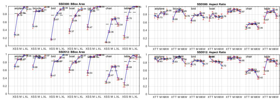
The authors also analyze how detection quality varies by object category, bounding box area, and aspect ratio. These diagnostics expose the kinds of errors the detector encounters, including localization errors, confusion with similar categories, and sensitivity to small objects or unusual aspect ratios. Such observations motivate the multi scale default box design, hard negative mining, and aggressive patch based augmentation. The category level diagnostics are shown in the figure below:

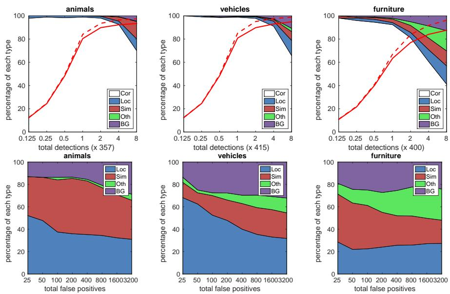
The size and aspect ratio diagnostics highlight that model behavior changes across object dimensions, especially for small bounding boxes and atypical aspect ratios. This guides the training procedure toward augmentation strategies that repeatedly expose the detector to varied cropping scales and spatial layouts.

Experiment

Experiments use a VGG16-based SSD architecture evaluated on PASCAL VOC2007 and VOC2012, COCO, and preliminary ILSVRC detection tasks. The main benchmarks show that SSD delivers competitive or superior detection accuracy against Fast R-CNN, Faster R-CNN, and YOLO while maintaining real-time inference. Additional model analyses validate the roles of data augmentation, diverse default box shapes, atrous convolutions, and multi-resolution feature maps, while an augmentation-based zoom-out strategy and timing results highlight improved small-object performance and efficient inference.

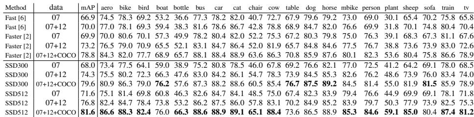
The VOC2007 test results show that adding more training data improves detection accuracy across methods, with the strongest gains seen when combining VOC2012 with COCO-based training for Faster R-CNN. SSD300 benefits markedly from the larger training set and becomes competitive with Faster R-CNN trained on VOC2007. The reported findings also indicate that larger input sizes and extra data help detection quality, especially for smaller objects. Fast R-CNN and Faster R-CNN both improve when trained on 07+12 rather than VOC2007 only. Adding COCO pretraining gives Faster R-CNN the strongest overall detection accuracy. SSD300 improves substantially with 07+12 training and approaches Faster R-CNN trained on VOC2007.

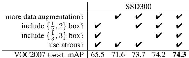
The results show that broader data augmentation, more diverse default box shapes, atrous convolutions, and predictions from multiple output layers all benefit SSD performance. Removing or reducing these components leads to lower accuracy or slower inference, with fewer output layers causing a monotonic decline in detection quality. More default box shapes improve detection accuracy by making box prediction easier. Atrous convolutions provide similar accuracy with faster inference than the full VGG16 variant.

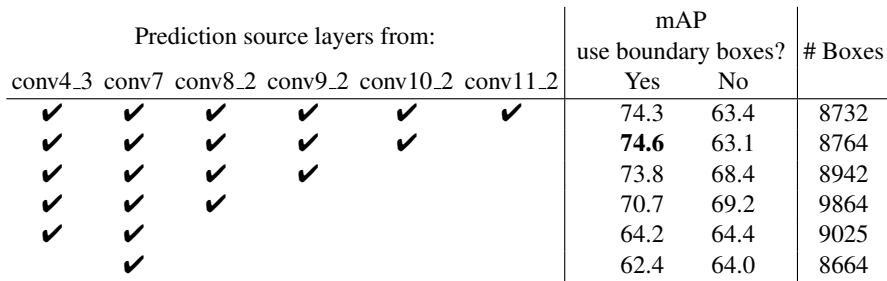
The results show that prediction sources from multiple output layers at different resolutions give higher detection accuracy than configurations with fewer layers, even when the total number of default boxes is kept roughly comparable. Accuracy falls progressively as output layers are removed. Using boundary boxes helps most in the full multi layer setting, while reduced layer settings show a much smaller benefit. Multiple prediction layers improve accuracy over using only a subset of layers. Boundary box handling is important in the full configuration, and its effect weakens as fewer layers are used.

On PASCAL VOC2012 detection, SSD300 is more accurate than Fast and Faster R-CNN trained on the same VOC data, and SSD512 gives a further accuracy gain from larger input resolution. The SSD models are much better than YOLO, while pretraining on COCO then fine-tuning on VOC improves both Faster R-CNN and SSD, with SSD512 reaching the strongest mAP. Higher input resolution from SSD300 to SSD512 improves detection accuracy. COCO pretraining and VOC fine-tuning increase mAP for Faster R-CNN and SSD. SSD is substantially more accurate than YOLO on VOC2012.

On COCO detection, SSD300 trained with adjusted default boxes outperforms Fast R-CNN on both mean average precision at 0.5 overlap and across 0.5 to 0.95 overlap. It is close to Faster R-CNN and ION on stricter IoU 0.75 while trailing them at IoU 0.5. Using a larger input scale in SSD512 yields larger gains on large objects than on small objects. SSD300 improves average precision over Fast R-CNN at both 0.5 overlap and the 0.5 to 0.95 overlap range. SSD300 has competitive precision at IoU 0.75 but lower precision at IoU 0.5 than Faster R-CNN and ION. The SSD512 comparison shows larger improvements for large object precision and recall than for small object metrics.

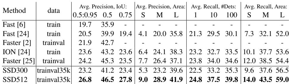
Experiments on PASCAL VOC and COCO compare detection models under varying training data, input resolutions, and architecture settings. They show that larger training sets, COCO pretraining, higher input sizes, richer augmentations, diverse default boxes, atrous convolutions, and multi-layer predictions improve detection quality, especially for small objects and stricter overlap thresholds. SSD is more accurate than YOLO, competitive with Faster R-CNN, and benefits from multi-layer default boxes, while larger inputs help more for large objects.