One-sentence Summary

University of Washington, Allen Institute for AI, and Facebook AI Research propose YOLO, which reframes object detection as a single-network regression problem that predicts bounding boxes and class probabilities directly from full images, achieving 45 FPS in real time and outperforming DPM and R-CNN in cross-domain generalization to artwork.

Key Contributions

• Introduces YOLO, a single convolutional network that reframes object detection as regression from full-image pixels to bounding box coordinates and class probabilities, enabling end-to-end optimization directly on detection performance.

• Demonstrates real-time detection with the base YOLO model running at 45 frames per second on a Titan X GPU and Fast YOLO reaching 155 frames per second while achieving more than twice the mAP of other real-time detectors.

• Shows that full-image context reduces background false positives to less than half those of Fast R-CNN, and that YOLO outperforms DPM and R-CNN when generalizing from natural images to artwork.

Introduction

The authors study object detection, a computer vision task where systems must identify what objects are present in an image, where they are located, and how they interact. This matters for applications such as autonomous driving, assistive vision devices, and responsive robotics, where fast and accurate perception is essential.

Prior detection methods mainly repurpose image classifiers by scanning many locations and scales, or by generating candidate regions before classification. These approaches often rely on complex, multi stage pipelines that must be trained separately, making them slower and harder to optimize. They can also struggle with background errors and limited contextual understanding.

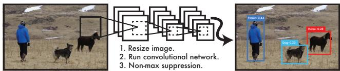
To address these challenges, the authors introduce YOLO, which reformulates object detection as a single regression problem. Using one convolutional network, it directly predicts bounding boxes and class probabilities from the whole image. This design enables real time performance, stronger use of global context, and better generalization to new domains, while still trading off some accuracy on precise localization, especially for small objects.

Method

The authors leverage a unified convolutional detector that replaces a multi stage detection pipeline with a single neural network. The model uses features from the full input image to predict bounding boxes and class probabilities simultaneously, which allows the network to reason about the whole scene rather than treating detection as a sequence of independent proposals and classifiers.

The image is divided into an $S \times S$S×S grid. If the center of an object falls into a grid cell, that grid cell is responsible for detecting the object. Each cell predicts $B$B bounding boxes along with confidence scores. The confidence score expresses both the probability that the cell contains an object and the expected accuracy of the predicted box:

If a cell contains no object, the desired confidence is zero. If it does contain an object, the confidence should approximate the intersection over union between the predicted box and the ground truth. Each box is represented by five values: center coordinates $(x,y)$(x,y), width $w$w, height $h$h, and confidence. The center coordinates are parameterized as offsets relative to the corresponding grid cell, while the width and height are normalized with respect to the whole image.

Each grid cell also predicts conditional class probabilities, $\Pr(\text{Class}_i|\text{Object})$Pr(Classi​∣Object). These probabilities are conditioned on the presence of an object in that cell. At inference time, the conditional class probabilities are multiplied by the box confidence to obtain a class specific score:

This score encodes both the likelihood that a class appears in the box and how well the predicted box matches the object. For a standard configuration with $S=7$S=7, $B=2$B=2, and $C=20$C=20, the network outputs a $7\times 7\times 30$7×7×30 prediction tensor.

The detector itself is implemented as a deep convolutional network. The early convolutional layers extract visual features, while the later fully connected layers produce the predicted probabilities and coordinates. The architecture contains 24 convolutional layers followed by 2 fully connected layers. Instead of using inception style modules, it alternates $1\times 1$1×1 reduction layers with $3\times 3$3×3 convolutional layers to control computational cost while preserving representational depth. The complete detector stack, from feature extraction to the final prediction tensor, is shown in the figure below:

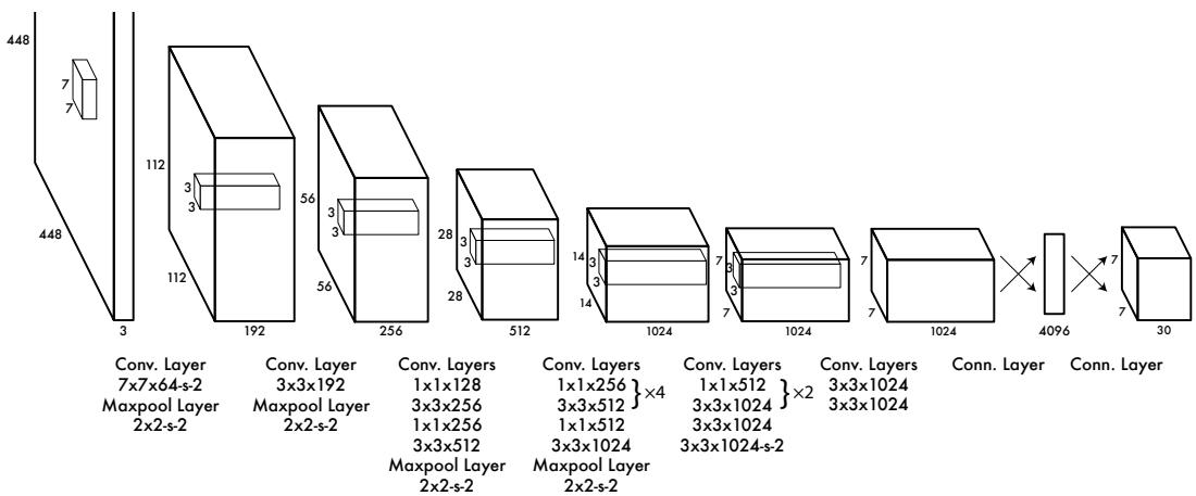
A faster variant is obtained by reducing the number of convolutional layers and the number of filters in those layers. In this reduced model, the remaining training and testing procedure is unchanged.

Training begins with classification pretraining. The convolutional backbone, typically the first 20 convolutional layers of the detection network, is trained on a large classification dataset with added average pooling and a fully connected output layer. The pretrained weights are then transferred to detection by adding randomly initialized convolutional and fully connected layers. Because detection requires finer spatial detail, the input resolution is increased before detection training. The final layer uses a linear activation, while all preceding layers use leaky rectified linear activation:

The network is optimized with a multi part sum squared error objective. A direct squared loss is easy to minimize, but it can be poorly aligned with detection performance because it equally weights localization error and classification error, and it can over penalize empty grid cells. To address this, coordinate errors are weighted more heavily, while confidence errors for non object cells are downweighted. The weighting parameters are set to $\lambda_{\text{coord}}=5$λcoord​=5 and $\lambda_{\text{noobj}}=0.5$λnoobj​=0.5. To reduce the disproportionate effect of localization error in small boxes, the model predicts the square root of box width and height:

Here, $\mathbb{1}_{i}^{\text{obj}}$1iobj​ indicates that an object appears in cell $i$i, and $\mathbb{1}_{ij}^{\text{obj}}$1ijobj​ indicates that the $j$jth box predictor in cell $i$i is responsible for that object. Responsibility is assigned to the box predictor that currently has the highest IOU with the ground truth. This encourages different box predictors to specialize in different object sizes, aspect ratios, or categories.

Training uses a batch size of 64, momentum of 0.9, and weight decay of 0.0005. The learning rate is warmed up from $10^{-3}$10−3 to $10^{-2}$10−2 to avoid early divergence, then follows a staged decay schedule. Dropout is applied after the first fully connected layer to reduce co adaptation between units. Data augmentation is performed by applying random scaling and translation of up to 20 percent of the original image size, along with random adjustments of exposure and saturation by up to a factor of 1.5 in HSV color space.

At test time, detection requires only a single forward pass through the network. The grid based prediction design enforces spatial diversity, so multiple cells may sometimes predict overlapping boxes for the same object, especially for large objects or objects near grid cell boundaries. Non maximum suppression is used to remove duplicate detections while preserving the final class specific confidence scores.

Experiment

The experiments evaluate YOLO on PASCAL VOC, analyze its errors against Fast R-CNN, test cross-domain generalization to artwork, and verify real-time webcam deployment. YOLO is shown to provide an efficient real-time detection framework, while Fast R-CNN remains accurate but makes more background false positives, and the complementary error patterns allow YOLO to rescore Fast R-CNN detections and reduce those false positives. YOLO also generalizes better than proposal-based detectors to artwork by modeling object shape and spatial context, supporting its practical use in interactive real-time applications.

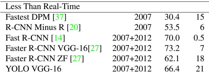
The table compares fast object detectors on PASCAL VOC 2007, highlighting YOLO as a detector that balances accuracy and speed well. Fast YOLO is described as the fastest detector while remaining substantially more accurate than other real-time systems, and the standard YOLO version improves accuracy over the fast version while still running well above real time. Fast YOLO is presented as the fastest detector with accuracy far above other real-time detectors. Standard YOLO trades some speed for a clear accuracy gain over Fast YOLO while remaining fast. YOLO stays competitive with Faster R-CNN variants while offering much higher throughput than the slower high accuracy detectors.

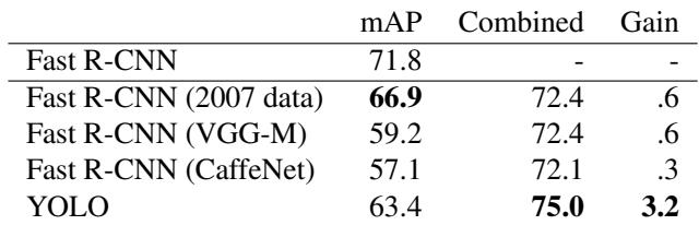
Combining the strongest Fast R-CNN with YOLO produces a notably larger gain on VOC 2007 than combining it with other Fast R-CNN variants. The improvement is attributed to YOLO making different mistakes, especially fewer background errors, rather than to generic model ensembling. Although both models are run separately, YOLO is fast enough that adding it does not introduce significant extra computation. YOLO gives Fast R-CNN a much larger performance boost than other Fast R-CNN models. Fast R-CNN ensemble combinations produce only small gains. The Fast R-CNN and YOLO combination adds little computational time because YOLO is fast.

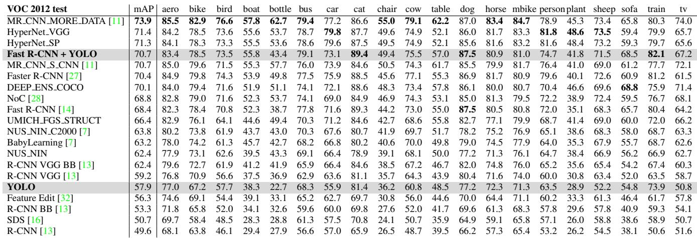
On PASCAL VOC 2012, standalone YOLO trails the leading detection methods, while the combined Fast R-CNN + YOLO model is among the highest-scoring systems. The combination gives Fast R-CNN a notable improvement and moves it up the public leaderboard. YOLO also shows category-specific strengths and weaknesses, with lower performance on some small-object classes and better performance on classes such as cat and train. Fast R-CNN + YOLO is among the top performing methods in the leaderboard comparison. The combination improves Fast R-CNN by 2.3% mAP and raises its leaderboard ranking. YOLO is described as the only real-time detector in this comparison. YOLO performs relatively worse on some small-object classes and better on classes such as cat and train.

YOLO achieves the strongest person detection results among the listed methods on both natural images and artwork datasets. Its performance degrades less than other detectors when moving from VOC 2007 to the Picasso and People-Art datasets, indicating better cross-domain generalization. R-CNN is competitive on VOC 2007 but drops substantially on artwork, while DPM transfers more stable but lower-accuracy performance. YOLO leads the compared detectors across the reported natural-image and artwork person detection settings R-CNN performs well on natural images but loses much more accuracy on artwork datasets DPM maintains more stable performance across artwork datasets than R-CNN but starts from a lower baseline

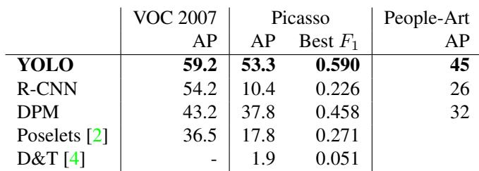
Experiments evaluate YOLO on PASCAL VOC 2007 and 2012 and in cross-domain person detection, assessing real-time speed, standalone accuracy, complementary ensembling, and robustness to domain shift. On VOC, fast and standard YOLO variants demonstrate that the detector balances speed and accuracy, while combining YOLO with Fast R-CNN yields a larger gain than other fast model combinations because the detectors make different mistakes. Although standalone YOLO trails leading methods on VOC 2012, the combined model performs strongly and shows class-dependent behavior, with weaker results on small objects; person detection results further indicate that YOLO generalizes better to artwork than several compared detectors.