One-sentence Summary

Researchers from the Institute for Artificial Intelligence, Peking University reveal the elasticity of post-alignment LLMs, demonstrating via compression theory that fine-tuning disproportionately undermines alignment relative to pretraining, and that elasticity correlates positively with model size and pretraining data scale.

Key Contributions

• The paper identifies elasticity in post-alignment LLMs, where further fine-tuning can cause behavior distributions formed during pretraining to reappear. This supports an alignment resistance mechanism that can reverse or diminish alignment.
• Using a compression-theoretic account of training and alignment, the work shows that changes in normalized compression rate under fine-tuning perturbations are inversely related to dataset size, so models tend to retain larger pretraining distributions and forget smaller alignment distributions.
• Experiments on LLMs of varying types and scales show rapid performance decline followed by reversion toward the pretraining distribution, with elasticity strengthening as model size and pre-training data volume increase.

Introduction

Large language models are widely deployed because they can generate fluent, general purpose text, but their ability to stay aligned with human intent and safety requirements is critical for real world use. In practice, models must balance broad utility with robust safety, making reliable alignment a core system design challenge.

Prior work has mainly relied on training based alignment methods such as supervised fine-tuning, reinforcement learning with human feedback, and related variants. Although these approaches reduce harmful behavior, they often appear superficial. Highly aligned models can quickly become unsafe after only light fine-tuning, and even benign task fine-tuning can weaken safety mechanisms. Existing analyses point to fragile alignment, but the underlying mechanism has remained unclear.

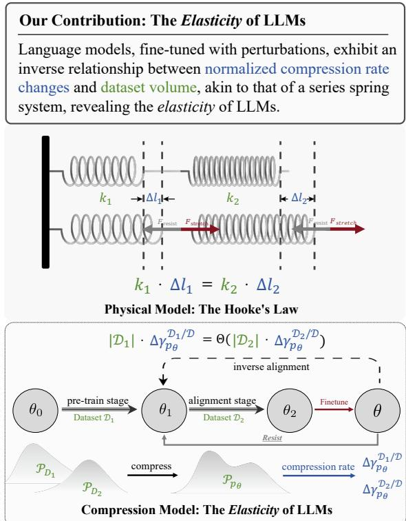
The authors identify elasticity as a key mechanism behind alignment fragility. They argue that language models resist changes to distributions learned from large pretraining datasets, while changes induced by smaller datasets can rebound more easily. Using compression theory, they model training and alignment as processes affecting the model’s normalized compression rate, showing that alignment perturbations may be reversed or undone through inverse fine-tuning. Their contribution is a theoretical and empirical account of why alignment is inherently unstable: pretraining distributions persist, stronger alignment can rebound faster, and model changes scale inversely with dataset size, making current alignment methods prone to erosion under small perturbations.

Method

The authors leverage the equivalence between predictive modeling and lossless compression to recast the training, alignment, and perturbation behavior of language models as a compression process over multiple data distributions. The proposed framework does not introduce a new network architecture; instead, it reframes the existing training pipeline as a sequence of compression events in which the language model parameters $\theta$θ act as a compression protocol. Pretraining establishes a broad base distribution, supervised fine tuning shifts that distribution toward an alignment target, and subsequent perturbations, such as reverse fine tuning, reveal whether the model can be driven back toward an earlier distribution. By measuring how efficiently the model compresses each relevant dataset, the method turns alignment resistance into an information theoretic quantity.

The starting point is the standard training objective for a language model. During pretraining, the model learns to predict tokens in long text sequences. For a prefix $\boldsymbol{x}=(x_0,\ldots,x_{N-1})$x=(x0​,…,xN−1​) from the pretraining corpus $\mathcal{D}_{\mathrm{PT}}$DPT​, the loss is

For supervised fine tuning, the model is trained on pairs $(\boldsymbol{x},\boldsymbol{y})$(x,y) drawn from a high quality alignment distribution $\mathcal{D}_{\mathrm{SFT}}$DSFT​, with objective

When the target distribution is fixed, minimizing this negative log likelihood loss is equivalent to minimizing the KL divergence between $p_{\boldsymbol{\theta}}$pθ​ and the desired SFT distribution. The compression view connects this directly to coding theory. If a model $p_{\boldsymbol{\theta}}$pθ​ is used inside arithmetic coding, the expected code length of a sequence $\boldsymbol{x}=(x_0,\ldots,x_{m-1})$x=(x0​,…,xm−1​) is

Thus, minimizing the training loss corresponds to minimizing the expected code length. In this formulation, training a language model and compressing its training distribution are treated as equivalent tasks.

To make the compression process explicit for sequential generation, the authors model each dataset as a token tree. For simplicity, the token vocabulary is assumed to contain only binary tokens, such as $0$0 and $1$1, along with an end of sequence marker. Each node in the token tree has two child edges labeled $0$0 and $1$1, and a leaf path ending with an EOS node represents one response in the dataset. The weight of a leaf node corresponds to the probability of that response, while the weight of an internal node is the sum of the weights of its descendants. Training the language model can then be interpreted as learning weights over portions of this infinite token tree.

Because a real model has finite parameters, it cannot represent the entire infinite token tree exactly. The method introduces the assumption that the model can perfectly model only a finite depth of the tree, and that this depth increases monotonically with model size. Given a parameterized model $p_{\boldsymbol{\theta}}$pθ​, the corresponding compression protocol is defined in two steps. First, the token tree for the relevant dataset is pruned, keeping only the top $d$d layers. Second, Huffman coding is applied to the pruned tree, where each complete root to leaf path is treated as a symbol in the coding alphabet. This yields an optimal and lossless compression procedure for the modeled portion of the data distribution.

The ideal expected code length for a response $\boldsymbol{x}$x compressed by the finite model is written as

where $d$d is the effective depth retained by the pruning step, and $p_{lj}$plj​ denotes the probability assigned to the $j$jth leaf node at depth $l$l under the compressed protocol. When multiple disjoint datasets are trained on jointly, the authors combine their token tree weights according to dataset size. For datasets $\mathcal{D}_1,\ldots,\mathcal{D}_N$D1​,…,DN​, the combined node probability is

where $|\mathcal{D}_i|$∣Di​∣ is the size of dataset $\mathcal{D}_i$Di​. This construction allows the method to assign a compression rate to each individual dataset under the same trained model. The dataset specific compression rate is

A normalized compression rate is then introduced to compare datasets of different structure and leaf counts. If $\mathcal{T}_i'$Ti′​ is the pruned tree for dataset $\mathcal{D}_i$Di​ and $M$M is the number of its leaf nodes, the normalized rate is

Smaller normalized compression rates indicate stronger alignment between the model distribution and the target dataset distribution. This metric becomes the central observable for studying whether alignment is stable after perturbation.

The formal inverse alignment definition uses this metric. Suppose a base model $p_{\boldsymbol{\theta}_0}$pθ0​​ is aligned on dataset $\mathcal{D}_a$Da​ to produce $p_{\boldsymbol{\theta}_1}$pθ1​​. If applying a much smaller perturbation dataset $\mathcal{D}_b$Db​ yields a model $p_{\boldsymbol{\theta}_0'}$pθ0′​​ such that the behavioral or distributional distance satisfies

then the transition from $p_{\boldsymbol{\theta}_1}$pθ1​​ back toward $p_{\boldsymbol{\theta}_0'}$pθ0′​​ is called inverse alignment. In the compression framework, $\rho$ρ is instantiated by the compression rate, so alignment reversal can be analyzed by tracking changes in $\gamma_{p_{\boldsymbol{\theta}}}^{\mathcal{D}_i/\mathcal{D}}$γpθ​Di​/D​ rather than relying only on behavioral benchmarks.

The core analytical pipeline separates three data roles: $\mathcal{D}_p$Dp​ for pretraining, $\mathcal{D}_a$Da​ for alignment, and $\mathcal{D}_t$Dt​ for perturbation. The method assumes that alignment and perturbation distributions can be viewed as subsets or reweighted versions of the broader pretraining data distribution. Under a Pareto type mass distribution assumption, the authors derive an inverse proportionality law between changes in normalized compression rate and dataset size. With

the result is

with

This means that as perturbation data is added, the model becomes more compressible on the larger pretraining distribution and less compressible on the smaller alignment distribution. The method interprets this as a bias toward large data volume: the model behaves as if resources in the compression protocol are preferentially allocated to the larger distribution. This asymmetry explains why alignment can be shallow and why small perturbations can erase it.

The method then maps this behavior onto a physical invariant analogous to Hooke’s law. In a series spring system with spring constants $k_1$k1​ and $k_2$k2​, an external force produces deformations $\Delta l_1$Δl1​ and $\Delta l_2$Δl2​ such that

In the language model setting, dataset size $|\mathcal{D}_i|$∣Di​∣ plays the role of spring stiffness, while the change in KL divergence

plays the role of deformation. The resulting elastic quantity satisfies

As shown in the figure below:

Under this formulation, pretraining distribution $\mathcal{P}_{\mathcal{D}_1}$PD1​​, alignment distribution $\mathcal{P}_{\mathcal{D}_2}$PD2​​, and final model distribution $\mathcal{P}_{p_{\boldsymbol{\theta}}}$Ppθ​​ are all represented through compression rates. The top part expresses the physical analogy, where stiffer components deform less, while the bottom part expresses the model behavior: after perturbation, changes in normalized compression rate are inversely related to dataset volume. The framework therefore represents inverse alignment as the consequence of a distributional preference for large volume data under compression dynamics. Resistance appears when a pretraining distribution remains dominant during alignment, and rebound appears when a fine tuned model shifts back toward that larger original distribution under reverse fine tuning.

Experiment

the paper experimentally evaluate language-model elasticity by comparing forward and inverse alignment on successive SFT slices across several Llama models and datasets, testing rebound after positive-to-negative fine-tuning, and analyzing how rebound varies with model size and pre-training data volume. The results show that inverse alignment is consistently easier than forward alignment, supporting the existence of resistance, while models aligned more strongly on positive data exhibit stronger rebound when exposed to opposing data before stabilizing. Further analyses indicate that rebound becomes more pronounced as model parameter count and pre-training data increase, suggesting greater elasticity in larger, more extensively pre-trained models.

Across the tested base models and datasets, forward alignment consistently produces higher training loss than inverse alignment. This gap appears for all compared stage transitions, indicating that models more easily recover from later-stage responses to earlier-stage responses than the reverse. The pattern suggests that pre-trained models tend to preserve their original distribution and resist alignment updates. Inverse alignment loss is lower than forward alignment loss across Alpaca, TruthfulQA, and safety task settings. The resistance pattern remains consistent across Llama2 and Llama3 models and different slice pair selections.

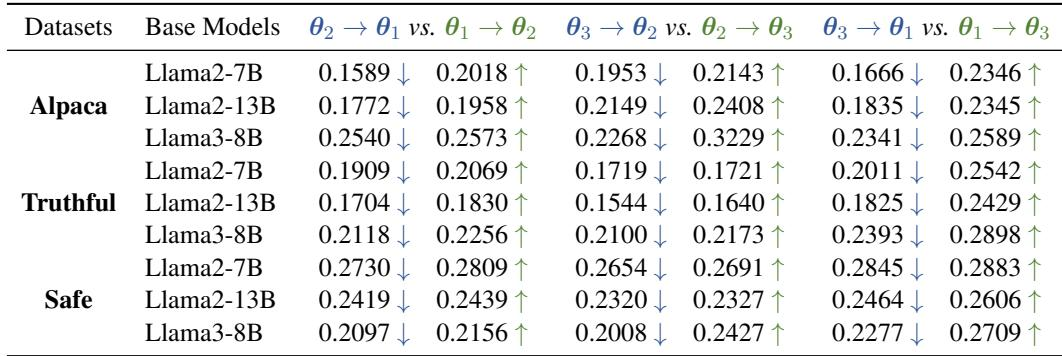
Experiments compare forward and inverse alignment training losses across multiple Llama2 and Llama3 settings, showing that inverse alignment consistently produces lower loss than forward alignment. This suggests that pre-trained models more easily transition from later-stage responses back to earlier-stage responses than the reverse, reflecting a tendency to preserve their original distribution and resist alignment updates. The pattern remains consistent across Alpaca, TruthfulQA, safety tasks, and different slice pair selections.