One-sentence Summary

Researchers at Meijo University introduce observed-block multiprediction for Deep Boltzmann Machines in statistical data fusion, showing that cross-block conditioning when predicting one outcome block from the other provides a small yet persistent gain ($+0.07\text{--}0.19$+0.07–0.19 percentage points) across all sample sizes and covariate widths, in contrast to generative pre-training, whose benefit decays.

Key Contributions

• Observed-block multiprediction (OBMP) is proposed as a discriminative training criterion that restricts multi-prediction to targets each row actually observes, making it well-defined for data fusion with disjoint outcome blocks and reducing to the standard criterion when rows are complete.
• On two consumer panels across 35 grid cells and 875 runs, a Deep Boltzmann Machine fine-tuned with OBMP outperforms fifteen methods. Decomposition shows the advantage comes from a cross-block conditioning term (worth +0.19 and +0.07 percentage points, positive in all cells) rather than from generative pre-training.
• The cross-block term does not decay with sample size or model depth and is structurally inaccessible to purely discriminative models, clarifying that the unique contribution of joint models in data fusion is the ability to condition on one outcome block when predicting the other.

Introduction

The recent resurgence of energy-based models has renewed interest in the Deep Boltzmann Machine (DBM), a classical deep EBM whose native ability to handle partial observations makes it a natural fit for statistical data fusion. In this setting, two panels share a common covariate block but never observe both outcome blocks together, so any model of the joint distribution must learn associations without paired examples. Prior work either relied on a generative training objective that marginalizes missing dimensions, which yields weak predictors, or on discriminative multi-prediction training, which requires observed targets and is therefore impossible when no row contains both outcome blocks. The authors close this gap by introducing observed-block multi-prediction (OBMP), a discriminative criterion that restricts targets to what each row actually observes, enabling DBMs to be trained discriminatively in the fusion regime. They further decompose the model’s advantage, showing that the persistent gain comes from conditioning on one outcome block when predicting the other, a structural benefit that purely discriminative models cannot replicate.

Dataset

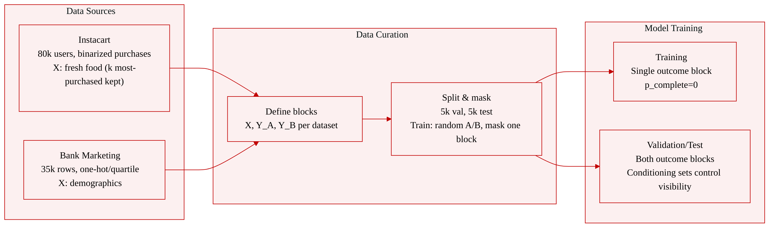
The authors use two datasets with deliberately different block geometries to evaluate the fusion setting. Both are split into three blocks: a visible block X and two outcome blocks Y_A and Y_B. No training example ever sees both outcome blocks; validation and test examples retain both for scoring.

• Instacart (online grocery panel)

  • Source: Binarized purchase indicators at the aisle level, drawn from a pool of 80,000 users.
  • Block composition:
    • X: Fresh-food departments (produce, dairy/eggs, beverages, bakery, meat/seafood). Only the k most-purchased aisles are kept; the rest are dropped entirely rather than moved to an outcome block.
    • Y_A: Ambient-food departments (pantry, frozen, snacks, breakfast, canned goods, dry goods, deli), 53 dimensions.
    • Y_B: Nonfood departments (personal care, household, babies, pets, alcohol, international, bulk, other), 46 dimensions.
    • Total visible dimensions: k + 99.
  • Split: 5,000 validation and 5,000 test users are held out from the 80,000-user pool.

• Bank Marketing (telemarketing records)

  • Source: A non-behavioral panel of 35,000 rows, with block geometry roughly the reverse of Instacart’s.
  • All variables are one-hot or quartile encoded.
  • Block composition:
    • X: Demographics (age quartiles, occupation, marital status, education).
    • Y_A: Financial standing (default flag, balance quartiles, housing and personal loans), 7 dimensions.
    • Y_B: Campaign contact history (contact channel, day/season, call-duration quartiles, contact and previous-contact counts, previous outcome, subscription flag), 29 dimensions.
    • Total visible dimensions: k + 36.
  • Split: 5,000 validation and 5,000 test rows.

• Data usage in training

  • Each training row is randomly assigned to source A or B with probability 0.5 and masked accordingly (only one outcome block is observed).
  • The probability of a row being complete (observing both outcome blocks) is set to zero; this is the regime that motivates the OBMP criterion.
  • Validation and test rows keep both outcome blocks, but conditioning sets control which block the model is allowed to see during prediction.

Method

The authors propose a fine-tuning strategy for Deep Boltzmann Machines (DBMs) tailored to data-fusion settings where no training row is fully observed. The core idea is an observed-block multi-prediction (OBMP) criterion that restricts the discriminative training signal to genuinely observed entries, enabling gradient flow from every row even when entire outcome blocks are missing. The method consists of a two-stage pipeline: a mask-aware generative pre-training stage followed by OBMP fine-tuning, both using the same DBM architecture and a differentiable unrolled mean-field inference procedure.

The DBM is defined with one visible layer $\mathbf{v} \in \{0,1\}^{D_v}$v∈{0,1}Dv​ and $L$L hidden layers $\mathbf{h}^{(1)},\dots,\mathbf{h}^{(L)}$h(1),…,h(L), each a binary vector. The joint energy follows the standard Bernoulli–Bernoulli parametrization:

with parameters $\theta = \{\mathbf{a}, \mathbf{b}^{(1:L)}, W^{(0:L-1)}\}$θ={a,b(1:L),W(0:L−1)}. Each training sample $i$i carries a binary observation mask $\mathbf{m}_i \in \{0,1\}^{D_v}$mi​∈{0,1}Dv​, where $m_{ij}=1$mij​=1 indicates that visible dimension $j$j is observed. In data fusion, the visible dimensions partition into three blocks: a common covariate block $X$X observed in every row, and two outcome blocks $Y_A$YA​ and $Y_B$YB​ observed in disjoint panels. Thus $\mathbf{v} = (\mathbf{x}, \mathbf{y}_A, \mathbf{y}_B)$v=(x,yA​,yB​), and a row’s mask is either $\mathbf{1}_X + \mathbf{1}_{Y_A}$1X​+1YA​​ (source A), $\mathbf{1}_X + \mathbf{1}_{Y_B}$1X​+1YB​​ (source B), or the all-ones vector for complete rows. The regime of interest is $p_{\text{complete}} = 0$pcomplete​=0, i.e., no row contains both outcome blocks.

Stage one: generative pre-training. The model is first trained with a mask-aware marginal log-likelihood that remains well-defined for any observation pattern:

Missing visible dimensions are summed out, so the criterion is purely generative and does not distinguish covariates from outcomes. The gradient is approximated using a factorized mean-field posterior for the positive phase and persistent contrastive divergence for the negative phase:

The visible bias is initialized from the observed marginals computed over entries where $m_{ij}=1$mij​=1, since no complete subset exists for layer-wise pre-training. The resulting model, called ML-DBM, serves as the initialization for the second stage.

Observed-block multi-prediction (OBMP). The original multi-prediction DBM (MP-DBM) draws a random subset of visible dimensions as prediction targets and requires ground-truth values for those entries, which is impossible when a row lacks entire outcome blocks. OBMP overcomes this by restricting targets to the observed set. For each row, two binary masks are introduced: a conditioning mask $\mathbf{c}_i$ci​ marking the entries supplied to inference, and a target mask $\mathbf{t}_i$ti​ marking the entries whose known values define the loss, subject to

The first constraint prevents a target from being used as evidence; the second ensures every target is genuinely observed. Entries that are neither conditioned on nor targeted are marginalized.

Let $\boldsymbol{\mu}^{(v)}(\mathbf{c}_i) \in [0,1]^{D_v}$μ(v)(ci​)∈[0,1]Dv​ denote the visible marginals returned by the mean-field procedure when the entries selected by $\mathbf{c}_i$ci​ are clamped to their observed values. The OBMP criterion is the per-row normalized binary cross-entropy:

where $\ell(p,y) = -y\log p - (1-y)\log(1-p)$ℓ(p,y)=−ylogp−(1−y)log(1−p) and $\mathcal{I} = \{i : \sum_j t_{ij} > 0\}$I={i:∑j​tij​>0}. The inner normalization weights every row equally regardless of how many targets it contributes, preventing panels with wider outcome blocks from dominating the gradient. In practice, $\boldsymbol{\mu}^{(v)}$μ(v) is clamped to $[\varepsilon, 1-\varepsilon]$[ε,1−ε] before the logarithm.

OBMP is a strict generalization of MP-DBM: when all rows are complete and the masks are random complements, the two criteria coincide. Crucially, because targets are drawn from what each row actually observes, every row contributes gradient even when $p_{\text{complete}}=0$pcomplete​=0.

In the general case, the masks are obtained by splitting the observed set at random: a per-row keep probability $\pi_i \sim \mathcal{U}(\pi_{\min}, \pi_{\max})$πi​∼U(πmin​,πmax​) is drawn, each observed entry is kept independently with probability $\pi_i$πi​ to form $\mathbf{c}_i$ci​, and the rest become targets:

Data-fusion instantiation. For the fusion setting, the authors replace the random split with a deterministic one that mirrors the deployment pattern. They condition on the common block $X$X and target every observed outcome:

Thus a source-A row targets $Y_A$YA​, a source-B row targets $Y_B$YB​, and a complete row targets both. This choice makes the criterion identifiable under the missingness regime of data fusion: missingness is determined by the source indicator, which is independent of the outcome values given $X$X, so the objective targets $p(\mathbf{y}_A \mid \mathbf{x})$p(yA​∣x) on source-A rows and $p(\mathbf{y}_B \mid \mathbf{x})$p(yB​∣x) on source-B rows, both identified from the observed data. The joint $p(\mathbf{y}_A, \mathbf{y}_B \mid \mathbf{x})$p(yA​,yB​∣x) is never required during training.

Differentiable mean-field unroll. To make $\boldsymbol{\mu}^{(v)}$μ(v) differentiable with respect to $\theta$θ, the authors unroll the mean-field inference for a fixed number of passes $T$T and backpropagate through the entire computation. The initialization clamps the conditioned entries and sets the remainder from the visible bias, then propagates upward:

with $\boldsymbol{\mu}^{(0),\tau} := \boldsymbol{\mu}^{(v),\tau}$μ(0),τ:=μ(v),τ. Each subsequent pass $\tau = 1,\dots,T$τ=1,…,T updates the visible marginals from the first hidden layer, re-clamps the conditioned entries, and sweeps the hidden layers bottom-up:

The top-down term uses the previous pass’s marginals because the sweep proceeds bottom-up. Conditioned entries are never updated, so clamping is exact at every pass. The final visible marginals $\boldsymbol{\mu}^{(v)} := \boldsymbol{\mu}^{(v),T}$μ(v):=μ(v),T are used in the OBMP loss. Because the unroll is a composition of affine maps and logistic nonlinearities, the gradient of the loss flows through all $T$T passes, training the parameters for the inference procedure that will be used at test time.

Two-stage training procedure. Stage one fits the ML-DBM by optimizing the generative criterion (4) on all training rows. Stage two initializes from the stage-one parameters and minimizes the OBMP criterion (6) with the fusion split (13), selecting the checkpoint based on validation performance. The model architecture and the mean-field procedure remain unchanged; only the training objective shifts from generative to discriminative.

Inference-time conditioning. A single OBMP checkpoint supports multiple conditioning modes. In cross-block conditioning, to predict $Y_A$YA​ the model clamps everything else the row observes, including $Y_B$YB​: $\mathbf{c} = \mathbf{1}_X + \mathbf{1}_{Y_B}$c=1X​+1YB​​. Symmetrically, predicting $Y_B$YB​ uses $\mathbf{c} = \mathbf{1}_X + \mathbf{1}_{Y_A}$c=1X​+1YA​​. In X-only conditioning, both outcome blocks are hidden: $\mathbf{c} = \mathbf{1}_X$c=1X​, matching the training conditioning. The gap between these two modes isolates the value of conditioning on one outcome block when predicting the other, a quantity supplied entirely by the generative structure of the joint model since the two blocks are never observed together during training.

Experiment

The experiments evaluate a joint model (OBMP) for data fusion on two datasets, varying training set size and shared covariate width, and compare it against discriminative baselines and imputation methods. The primary advantage stems from cross-block conditioning at inference time, which leverages the association between outcome blocks to improve predictions, and this contribution remains positive and does not decay with sample size. Generative pre-training offers only a transient benefit that vanishes as more data becomes available, and the cross-block effect does not depend on a deep architecture, making it a structural advantage unavailable to models that rely solely on shared covariates.

In a statistical data fusion task with two outcome blocks, most performance improvements over baselines shrink as training data increases. The cross-block term, however, remains stable, indicating it captures structural information that models mapping covariates to outcomes cannot access. The overall effect is small, but its non-decaying nature distinguishes it from other diminishing margins. The cross-block term does not shrink with more training data, unlike other gains that decay. On one outcome block, the baseline model cannot outperform a constant predictor, leaving little room for improvement.

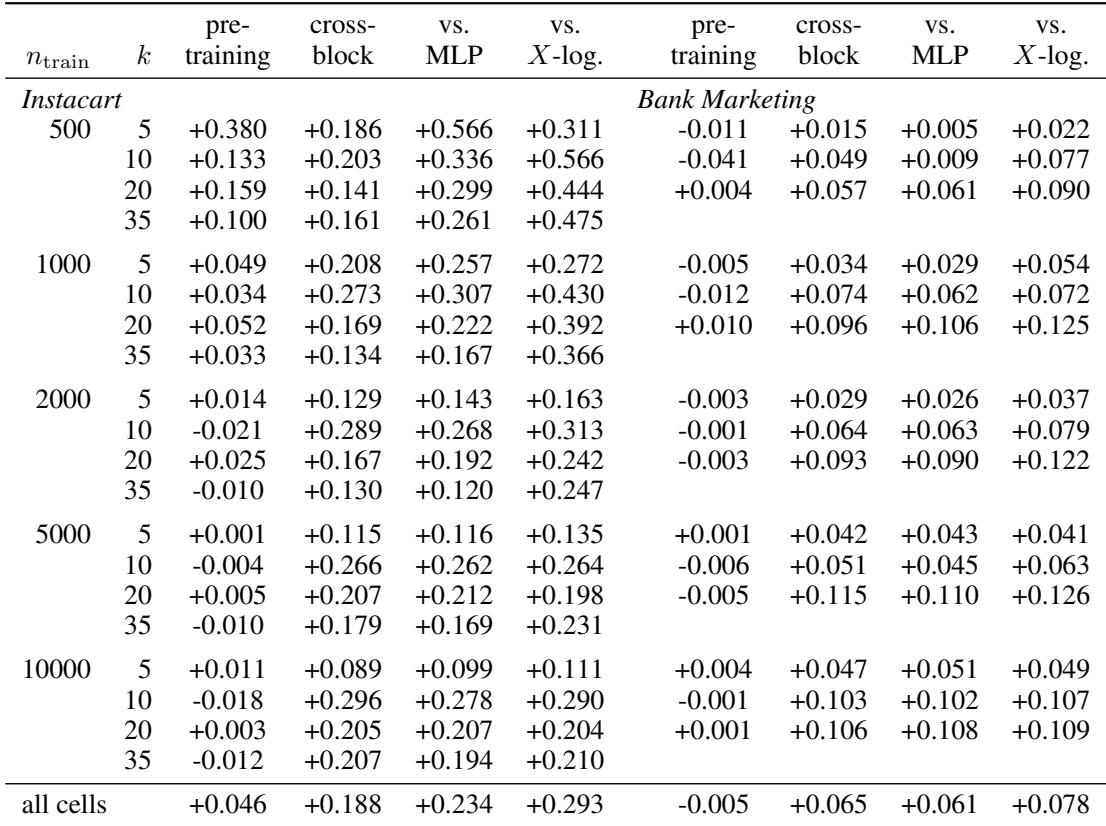
OBMP with cross-block conditioning achieves the highest combined accuracy across all training sizes and covariate sets on both datasets. Its advantage over baselines and ablations is widest in low-resource settings and narrows as training data grows, but never reverses. The generative model alone performs near a constant baseline, confirming that the gains stem from the cross-block conditioning rather than the generative stage. OBMP with cross-block conditioning is the top method in every cell, with the largest margins at the smallest training size. Cross-block conditioning consistently outperforms X-only conditioning, while the standalone generative model (ML-DBM) barely exceeds a constant predictor.

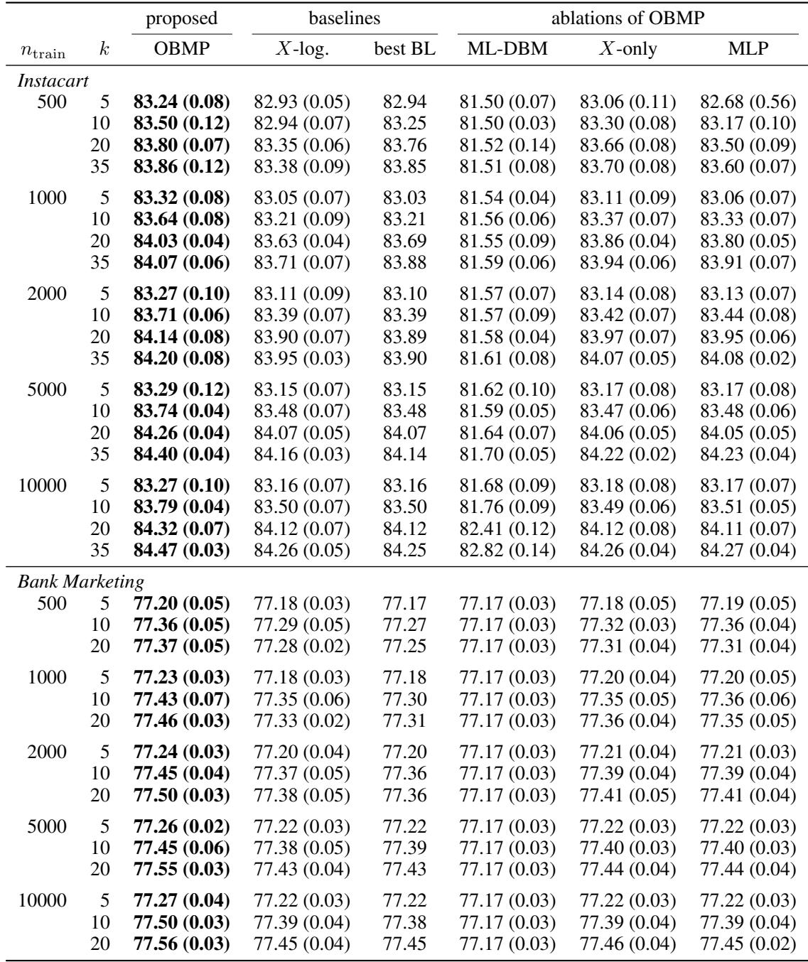
OBMP consistently outperforms all imputation baselines on both datasets, with positive paired differences in every comparison and statistically significant margins. The smallest gaps are against X-logistic and MICE, while the largest are against simple methods like column mean and k-NN. OBMP wins the vast majority of individual runs, losing at most a handful to any single baseline. OBMP's advantage is smallest against X-logistic and largest against column mean and k-NN across both datasets. OBMP wins at least 96 out of 100 Instacart runs and 73 out of 75 Bank Marketing runs against any imputation baseline.

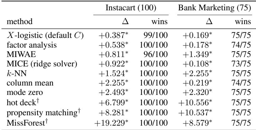
Generative pre-training offers little benefit over a discriminatively trained network of the same capacity once enough training data is available, with its contribution concentrated at the smallest sample size and vanishing elsewhere. In contrast, cross-block conditioning consistently improves accuracy in every tested configuration on both datasets, and its gain does not shrink with more data. The cross-block term captures associations between outcomes that are never observed together, a structural advantage that models mapping only covariates to outcomes cannot replicate. Cross-block conditioning yields positive accuracy gains in every single cell across both Instacart and Bank Marketing grids. Generative pre-training's contribution is almost entirely limited to the smallest training size (n_train=500) and becomes negligible with more data. On Bank Marketing, generative pre-training contributes essentially zero overall, averaging −0.005 pp across all runs. The cross-block advantage does not decay with increasing training samples, unlike the pre-training advantage. The cross-block term exploits outcome associations that were never fitted from paired data, propagated through shared hidden layers of the joint model.

When the association between outcome blocks is broken by permuting rows of one block, the cross-block conditioning term drops from a positive contribution to near zero and then becomes slightly negative, closely tracking the mean absolute between-block correlation. The generative pre-training contribution remains flat across all permutation levels, confirming that the cross-block term specifically captures the dependence between the two outcome blocks. The cross-block term falls from +0.178 pp with intact association to -0.029 pp when the blocks are fully independent, crossing zero near 50% permutation. Generative pre-training is unchanged across all permutation fractions, staying within ±0.01 pp, while the cross-block term moves systematically with the manipulated correlation. Permuting one outcome block causes only negligible collateral damage to the X-only logistic arm (0.048 pp), so the loss in overall performance is almost entirely due to the cross-block channel.

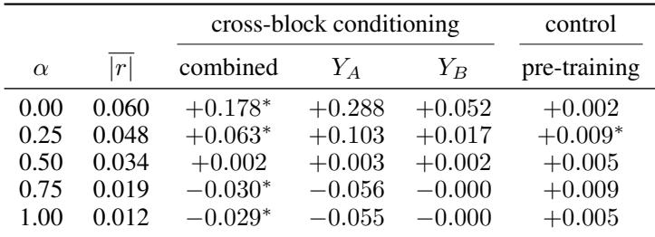
In a statistical data fusion task with two outcome blocks, the proposed OBMP model with cross-block conditioning consistently outperforms baselines, with the largest gains in low-data settings. The cross-block term captures structural associations between outcomes that are never observed together, and its advantage does not decay with more training data, unlike generative pre-training whose benefit vanishes as sample size grows. Breaking the outcome association by permutation eliminates the cross-block gain, confirming it relies on between-block dependence.