Command Palette
Search for a command to run...
Attention à poids rapides pour l'apprentissage continu
Attention à poids rapides pour l'apprentissage continu
Résumé
Les mémoires récurrentes à poids rapides et les modèles d'espace d'état sélectifs compressent un contexte en expansion en un état récurrent de taille fixe, faisant de la transition d'état une règle d'apprentissage en ligne. Nous étudions cette règle sous une sémantique autorégressive de lecture-après-écriture. Pour l'objectif de prédiction de préfixe considéré ici, l'exemple de mémoire rapide locale révélé à l'étape t est la paire alignée sur le préfixe (xt,yt) = (ϕ(kt−1),vt) . L'association courante à la même étape (ϕ(kt), vt) reste causale, mais optimise un objectif interne différent. Nous dérivons des mises à jour normalisées de premier ordre pour les objectifs de régression par erreur quadratique et de produit scalaire négatif. La famille de régression comprend Falcon-1 (une mise à jour NLMS scalaire), Falcon-2 (son extension par colonne) et Falcon-3 (une mise à jour par mini-lots à fenêtre glissante) ; Falcon-1A/Falcon-2A/Falcon-3A sont les variantes correspondantes de produit scalaire. Nous fournissons des formes récurrentes, parallèles masquées et parallèles par blocs, ainsi qu'une renormalisation à décroissance positive numériquement stable. Les variantes représentatives restent compétitives en modélisation du langage et améliorent l'extrapolation de longueur sur l'addition de chiffres variables. Ce cadre sépare l'alignement temporel, la plasticité, l'oubli et la répétition bornée dans les modèles séquentiels récurrents.
One-sentence Summary
Researchers from Bytedance Seed, Princeton, Tsinghua, UCLA, and Hyperbolic Labs propose a fast-weight attention framework for continual learning that derives normalized first-order updates for squared-error regression and negative inner-product objectives, introducing Falcon-1/2/3 variants (with inner-product counterparts Falcon-1A/2A/3A) that remain competitive in language modeling and improve length extrapolation on variable-digit addition.
Key Contributions
- Introduces a unified family of normalized fast-weight updates, Falcon-1/2/3 for squared-error regression and Falcon-1A/2A/3A for negative inner-product objectives, derived under read-after-write autoregressive semantics with prefix-aligned causal pairs (φ(kₜ₋₁), vₜ).
- Provides recurrent, masked-parallel, and chunk-parallel implementations with numerically stable positive-decay renormalization, separating temporal alignment, plasticity, forgetting, and bounded rehearsal while remaining compatible with SSD-style chunk-parallel training.
- Shows that representative scalar regression and scalar/sliding inner-product variants remain competitive in language modeling, and the best inner-product variants improve length extrapolation on variable-digit addition.
Introduction
Transformers dominate modern language modeling because self-attention captures global dependencies, but their quadratic scaling in sequence length creates major bottlenecks in both compute and memory, especially for long contexts. Recurrent alternatives like SSMs and fast-weight models compress memory into a fixed state, yet their state-update rules are often presented at the architectural level, leaving the underlying learning objective implicit. This ambiguity causes a temporal alignment mismatch: many recurrences bind the same-step pair (key, value), whereas autoregressive prediction requires pairing the newly revealed target with the prefix feature available at prediction time, a distinction that affects how fast memory is trained.
The authors address this by recasting state-based sequence modeling as autoregressive next-latent prediction, making the fast-memory training objective explicit. They derive a unified family of normalized first-order updates, Falcon-1, Falcon-2, and Falcon-3, along with inner-product counterparts, Falcon-1A, Falcon-2A, and Falcon-3A, which separate temporal alignment, plasticity, forgetting, and bounded rehearsal. These updates remain compatible with chunk-parallel training, and the authors provide implementations and empirical evaluations showing competitive language modeling performance and improved arithmetic length extrapolation.
Method
2 Background
2.2 Linear Attention
Linear attention circumvents the O(N2) complexity of standard attention by replacing the softmax with a kernel feature map ϕ(⋅):Rd→Rm such that κ(qt,kj)=ϕ(qt)⊤ϕ(kj). Exploiting the associativity of matrix multiplication, the output ot∈Rdv for the t-th token is:
ot=∑j=1tϕ(qt)⊤ϕ(kj)∑j=1tϕ(qt)⊤ϕ(kj)vj=ϕ(qt)⊤∑j=1tϕ(kj)(∑j=1tϕ(kj)vj⊤)⊤ϕ(qt),This formulation allows the context to be compressed into a recurrent matrix state St∈Rm×dv and a normalizer zt∈Rm:
ot=zt⊤ϕ(qt)+εattnSt⊤ϕ(qt),St=St−1+ϕ(kt)vt⊤,zt=zt−1+ϕ(kt).For a fresh sequence, Eq. (2.2) is exactly equivalent to Eq. (2.1) when S0=0, z0=0, εattn=0, and the denominator is nonzero. With εattn>0, it is the usual stabilized positive-feature variant. The normalized form is attention-like only when the read normalizer is nonnegative; signed-feature caveats are deferred to Appendix C.2.
Causality and indexing. Eq. (2.2) follows the standard Transformer convention: at position t the paper read from the updated state (St,zt), and the resulting representation is used to predict token t+1. The authors' next-latent alignment shifts the write stream by one: after observing vt, it is written under the previous write feature ϕ(kt−1), or equivalently, (ϕ(ki),vi+1) under standard indexing with i=t−1. This yields the read-after-write recurrence:
ot=zt⊤ϕ(qt)+εattnSt⊤ϕ(qt),St=St−1+ϕ(kt−1)vt⊤,zt=zt−1+ϕ(kt−1),where εattn≥0 is a small stabilizer. Defining the shifted write-feature stream:
x1:=0,xt:=ϕ(kt−1)for t≥2,Eq. (2.3) is exactly Eq. (2.2) with the standard write-feature stream {ϕ(kt)}t=1T replaced by {xt}t=1T when εattn=0; for εattn>0, it is the corresponding stabilized shifted variant. The boundary condition is therefore imposed in feature space rather than raw-key space.
Normalized vs. unnormalized linear attention. The denominator in Eq. (2.1) uses the normalizer state zt to rescale the readout. Many SSM/SSD-style architectures instead drop the denominator (and zt) and use an unnormalized inner-product read:
ot=St⊤ϕ(qt),St=(1−ηtλt)St−1+ηtϕ(kt−1)vt⊤,with the unshifted convention recovered by replacing kt−1 with kt. In this denominator-free form, state magnitude and the effective memory timescale are controlled by explicit decay (e.g., λt>0) and/or gain control. Section 4.3 shows that the numerator-state update in Eq. (2.4) is exactly gradient descent on an inner-product objective. The auxiliary normalizer zt in the normalized variants is a separate bookkeeping state for the read denominator; it is not itself obtained from that objective.
Accordingly, Eq. (2.4) is the gradient-descent update for the inner-product objective in Section 4.3. When λt=0, the write is purely additive rank-one Hebbian learning; when λt>0, it is additive plus scalar shrinkage. As noted in Section 2.1, Mamba-2 proves that the no-normalizer recurrence is functionally equivalent to a specific class of SSMs under the SSD framework.
2.3 Delta Networks
Fast Weight Programmers and Delta Networks formulate sequence modeling as the online learning of a value-retrieval function. Let St−1∈Rd×dv denote the fast-weight state matrix. Instead of purely additive accumulation, standard Delta Networks employ an error-driven update derived from the gradient of the instantaneous squared error between the state's reconstruction of the current key and value:
ℓt(S):=21S⊤kt−vt22.Here, S⊤k represents the model's prediction of value vt given key k. The gradient with respect to the state is ∇Sℓt(S)=kt(S⊤kt−vt)⊤.
Delta rule. the paper denote the gradient step size by ηt; later, βt denotes a dimensionless normalized gain and ηt the induced step size. A single online gradient step gives:
St=St−1−ηtkt(St−1⊤kt−vt)⊤=(I−ηtktkt⊤)St−1+ηtktvt⊤.The rank-one factor performs a targeted shrinkage/edit along the current key direction; it becomes an orthogonal projection only when ηt=1/∥kt∥22. Gated Delta Networks add an explicit global decay gate; notation and comparison details are in Appendix C.3.
3 Autoregressive Next-Latent Prediction
In this section, the authors cast the recurrent write as an explicit online optimization problem. Under the read-after-write convention, the causal example revealed at step t pairs the newly observed target with the prefix write feature available when that target was predicted, namely xt=ϕ(kt−1) and yt=vt. Standard DeltaNet instead uses the same-step pair (ϕ(kt),vt); that pairing remains causal, but it corresponds to a different local fast-memory objective. The authors therefore model S as an online linear predictor from xt to yt and optimize an instantaneous ridge-regression loss:
ℓt(S)≜21S⊤xt−yt22+2λt∥S∥F2,where λt≥0 is a regularization coefficient. While full-batch minimization of the cumulative loss corresponds to the offline solution found in methods like MesaNet, efficient autoregressive modeling requires an online approximation. The authors therefore employ Online Gradient Descent (OGD).
Notation. In kernelized linear attention, the key that writes to memory is typically a feature vector ϕ(k)∈Rm rather than the raw key k∈Rd. All derivations in this section are interpreted with:
xt≡ϕ(kt−1)∈Rm,St∈Rm×dv,so xt is treated as the generic write feature. Queries used for retrieval, e.g. ϕ(qt) in linear attention, live in the same feature space but need not equal xt. Whenever a summary sentence informally refers to a pairing in raw-key space, the mathematically exact kernelized object is the corresponding write feature.
Implicit fast-memory objective. Eq. (3.1) is the instantaneous objective whose gradient step defines the fast-memory write rule; it is not an additional supervised loss beyond the outer autoregressive likelihood. During training, the authors differentiate through the update so that the slow weights (which produce (q,k,v) as well as βt,λt) learn representations and gates that make these local updates useful.
Indexing and causality conventions. The read-after-write (RAW) convention is used throughout: after token t is observed and written, the updated state St is read to predict token t+1. Under next-latent alignment, the causal write pair is therefore (ϕ(kt−1),vt), or equivalently (ϕ(ki),vi+1) under standard indexing. The authors set S0=0 and impose the feature-space boundary x1:=0. For update rules with explicit shrinkage, the boundary sentinel is also assigned η1:=0 (equivalently, α1=0,γ1=1 in the log-space notation); otherwise λ1>0 would decay a carried state even though no data pair is written. Detailed RAW/RBW and boundary conventions are deferred to Appendix C.5.
With this convention, the internal fast-memory prediction is yt:=St−1⊤xt, with residual rt=yt−yt. This is distinct from the model readout at position t, which under RAW uses the updated state St.
Fast memory as continual learning. The recurrent state is the fast memory updated within the forward pass; each token provides a local training pair (xt,yt). Across the family, βt controls plasticity and λt controls shrinkage/forgetting; the realized ηt depends on the local normalization statistic, which is smoothness-matched for regression and energy-based for the inner-product implementations.
3.1 Online Gradient Descent Update
The gradient of the instantaneous loss in Eq. (3.1) with respect to the state S is:
∇Sℓt(S)=xt(S⊤xt−yt)⊤+λtS.Applying a single gradient descent step with learning rate ηt yields the update rule:
St←St−1−ηt∇Sℓt(St−1)=St−1−ηt[xt(St−1⊤xt−yt)⊤+λtSt−1]=(1−ηtλt)St−1+ηtxtrt⊤,where rt≜yt−St−1⊤xt is the residual (prediction error). Note that, unlike standard Delta Networks, rt measures the discrepancy between the prediction from the previous write feature xt=ϕ(kt−1) and the current value vt.
This is gradient descent on the instantaneous ridge objective. With the normalized step size below, it becomes a normalized update. In the special case λt=0 and ε=0, it reduces exactly to the classical NLMS recursion; for ε>0, it is the usual stabilized NLMS variant. Specifically, the loss ℓt is Lt-smooth with respect to the Frobenius norm, with smoothness constant Lt=∥xt∥22+λt. To ensure numerical stability and scale robustness, the authors adopt the normalized step size:
ηt=∥xt∥22+λt+εβt,βt∈(0,2),ε≥0.The authors adopt the convention ηt:=0 when ∥xt∥22+λt+ε=0, and also at the boundary sentinel t=1 when x1=0 is used to denote "no causal pair." In analysis, ε=0 may be taken and Lt>0 assumed. In implementations, ε>0 is used for numerical robustness; any ε>0 only decreases ηt and therefore preserves the descent guarantees below.
Appendix C.6 records secondary implementation details, including the βt>1 sign-flip regime and the positive-decay interpretation of ridge shrinkage under log-space unrolling.
3.2 Analysis
The authors show that the normalized step size yields per-step descent in the instantaneous regularized objective ℓt, a basic local stability property. This statement is pointwise in t: it does not imply monotone decrease of the cumulative online loss ∑sℓs or of the outer autoregressive training objective.
Lemma 3.1 (Per-step Descent for Smooth Losses). Let f:Rdx×dv→R be L-smooth with respect to the Frobenius norm. For any step size η∈(0,2/L), the gradient step S+=S−η∇f(S) satisfies:
f(S+)≤f(S)−2η(2−ηL)∥∇f(S)∥F2.Proof. By L-smoothness, for any S and S′:
f(S′)≤f(S)+⟨∇f(S),S′−S⟩+2L∥S′−S∥F2.Set S′=S+=S−η∇f(S) and simplify.
Step-size parametrization. Choosing η=β/L with β∈(0,2) (hence requiring L>0) yields a decrease coefficient β(2−β)/(2L). For L>0, the stabilized choice η=β/(L+ε) with ε≥0 also lies in (0,2/L). When L=0, this interval is undefined; in the degenerate cases arising here (xt=0 and λt=0, or the corresponding windowed analogue), the gradient is zero, so the update is defined to be a no-op by setting η:=0.
3.3 Delta Networks as Regression
In this section, the authors interpret many previous fast weight models under this optimization framework. They observe that Delta Networks and Linear Attention can be viewed as gradient updates induced by specific online objective functions.
By substituting the regression assignments xt←ϕ(kt−1) and yt←vt, Eq. (3.3) recovers the functional form of the Delta Network update rule, but with the critical index shift:
St=Decay & Targeted Forget((1−ηtλt)Idx−ηtxtxt⊤)St−1+Writeηtxtyt⊤,xt=ϕ(kt−1),yt=vt.Here, the rank-one term xtxt⊤St−1 is the left Hessian action of the squared-error loss along the current write-feature direction. Intuitively, it reduces the component of the current predictor that acts on xt=ϕ(kt−1) before adding the new target yt=vt.
In contrast, replacing the regression (MSE) loss with the inner-product objective of Section 4.3 removes the residual term and yields an additive write. With the standard unshifted assignment (xt,yt)=(ϕ(kt),vt) (or (kt,vt) in the unkernelized case), this is the familiar Linear Attention / Mamba-2 accumulation. With the next-latent assignment (xt,yt)=(ϕ(kt−1),vt), it becomes the one-step-shifted variant used by the authors' methods (e.g., Falcon-3A in Section 4.5).
This regression perspective motivates a key algorithmic improvement that the authors analyze in Section 4: with objective-matched normalization, the rank-one regression step uses Lt=∥xt∥22+λt, while the sliding rule uses Lt(B)=λmax(Cˉt(B))+λt. This suggests that fixed learning rates are scale-mismatched for regression-style fast-weight updates; for inner-product writes, the same normalization is better viewed as a magnitude stabilizer than as a curvature requirement.
Appendix A.2 gives reference pseudocode for the sequential first-order online-ridge update.
4 Falcon: Fast Weight Attention
Fast-weight memories and linear-attention architectures can be interpreted as online models that update a recurrent memory during the forward pass, tracing back to classical fast-weight mechanisms and their modern instantiations in linear Transformers and Delta-style rules. In this section, the authors derive Falcon from two local objectives under the shifted ϕ(kt−1)vt alignment: squared-error regression and a negative inner-product objective. This yields normalized step sizes, explicit forgetting controls, and sliding-window variants.
Naming and formula summary. All variants use the same causal pair:
xt:=ϕ(kt−1),yt:=vt,x1:=0,η1:=0,and read after writing, ot=St⊤ϕ(qt). Let rt:=yt−St−1⊤xt and Diag(ηt) denote the diagonal matrix of per-column step sizes. The regression family is:
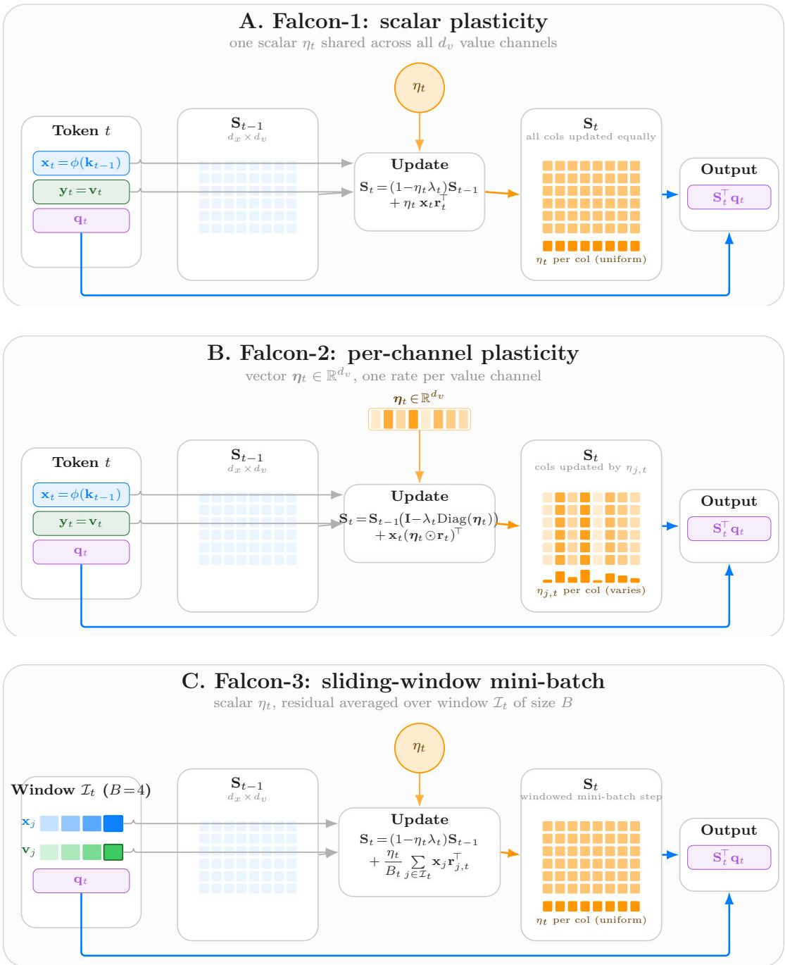
Falcon-1:St=(1−ηtλt)St−1+ηtxtrt⊤,ηt=∥xt∥22+λt+εβt, Falcon-2:St=St−1(Idv−λtDiag(ηt))+xt(ηt⊙rt)⊤,ηj,t=∥xt∥22+λt+εβj,t, Falcon-3:St=(1−ηtλt)St−1+Btηtj∈It∑xj(yj−St−1⊤xj)⊤,ηt=μt(B)+λt+εβt.Here μt(B)=λmax(Bt−1∑j∈Itxjxj⊤). The inner-product family replaces the residual regression write by direct target writes:
Falcon-1A:St=(1−ηtλt)St−1+ηtxtyt⊤,ηt=Et+λt+εβt, Falcon-2A:St=St−1(Idv−λtDiag(ηt))+xt(ηt⊙yt)⊤,ηj,t=Et+λt+εβj,t, Falcon-3A:St=(1−ηtλt)St−1+ηtNˉt(B),ηt=Eˉt(B)+λt+εβt,where Et=∥xt∥22, Nˉt(B)=Bt−1∑j∈Itxjyj⊤, and Eˉt(B)=Bt−1∑j∈It∥xj∥22. Thus, the index 1/2/3 denotes scalar, per-column, and sliding-window dynamics, respectively. The suffix "A" denotes the inner-product objective.
4.1 Scaled Linear Attention and Scaled DeltaNet
Unlike softmax attention, which uses the scaled dot product ⟨q,k⟩/d, fast-weight recurrences are directly sensitive to the norms of queries and keys: (i) dot-product reads grow with ∥qt∥2∥k∥2, and (ii) additive (inner-product) writes grow with the write-feature norm. To stabilize both the read and the write streams, especially under long decoding horizons and mixed precision, the authors use explicit feature scaling/normalization.
Scaled features. The authors define a generic RMS normalization operator for a vector u∈Rdu:
RMSNorm(u):=∥u∥22/du+εrmsu,where εrms>0 is a small stabilizer. Unless stated otherwise, RMSNorm is applied to the (qt,kt) projections used by fast-weight reads/writes, before forming dot products or outer products. This default differs from common ℓ2-normalized DeltaNet variants (e.g., in Gated DeltaNet implementations) and is substantially more stable in mixed precision because standard RMSNorm keeps coordinate magnitudes Θ(1). Moreover:
∥RMSNorm(u)∥22=∥u∥22+duεrmsdu∥u∥22≤du,so in the usual regime ∥u∥22≫duεrms the paper indeed have ∥RMSNorm(u)∥22≈du. By default, values vt are not normalized; value normalization (VNorm) is optional and disabled unless explicitly enabled.
Scaled Linear Attention. Under next-latent alignment, the RMS-normalized projections are used in the feature space. The scalar denominator-free inner-product recurrence, denoted Falcon-1A below, is:
ot=St⊤ϕ(qt),St=(1−ηtλt)St−1+ηtxtvt⊤,xt:=ϕ(kt−1).Its per-column counterpart, Falcon-2A, replaces the scalar write gain by a vector ηt∈Rdv:
St=St−1(Idv−λtDiag(ηt))+xt(ηt⊙vt)⊤.The corresponding normalized numerator/denominator recurrence is recorded in Appendix C.1; in signed-feature settings, the denominator caveat in Appendix C.2 applies.
Scaled DeltaNet and the common ridge parameterization. For regression-style fast weights, the same scaled write-feature xt is used inside the NLMS update:
St=(1−ηtλt)St−1+ηtxt(vt−St−1⊤xt)⊤,ηt=∥xt∥22+λt+εβt.In scaled implementations, the network may emit a dimensionless base ridge λˉt that is converted to the actual coefficient used by the recurrence, λt=λˉtEt, where Et is the appropriate normalization statistic: ∥xt∥22 for Falcon-2 and μt(B):=λmax(Cˉt(B)) for Falcon-3. The authors then set:
ηt=Et+λt+εβt,αt:=ηtλt,γt:=1−αt.Here Et=∥xt∥22 for the non-sliding scalar/per-column rules (Falcon-1/Falcon-2 and Falcon-1A/Falcon-2A), while Et=μt(B) for Falcon-3 and Et=E^t(B) for Falcon-3A. For regression, Et is the local smoothness scale of the data term; for inner-product writes, the corresponding energy statistics in Sections 4.3 and 4.5 are practical write-magnitude controls. Exact scale-robustness identities, detached-statistics details, the normalized linear-attention recurrence, and log-space positive-decay handling are deferred to Appendix C.1 and Appendix C.6.
4.2 Regression Loss (Delta Network)
The authors formulate the state update as an autoregressive linear regression problem. At time step t, let the state be St−1∈Rdx×dv, the write feature be xt≜ϕ(kt−1)∈Rdx, and the target be yt≜vt∈Rdv. (In the unkernelized case, ϕ is the identity and dx=d.) The state St−1 acts as a linear predictor mapping the prefix feature xt to the newly observed target yt.
The instantaneous squared-error loss is:
ft(S):=21S⊤xt−yt22.Evaluated at the pre-update state, the residual is rt≜yt−St−1⊤xt. The gradient with respect to the state is:
∇Sft(St−1)=xt(St−1⊤xt−yt)⊤=−xtrt⊤.Delta update (standard vs. next-latent). A single step of Online Gradient Descent (OGD) with learning rate ηt yields the Delta update:
St=St−1−ηt∇Sft(St−1)=St−1+ηtxtrt⊤=(Idx−ηtxtxt⊤)St−1+ηtxtyt⊤.Under next-latent alignment the paper have xt=ϕ(kt−1) and yt=vt. Replacing kt−1 with kt (equivalently, xt←ϕ(kt)) recovers the unshifted DeltaNet update of Schlag et al.
L2 Regularization. Adding an L2 penalty 2λt∥S∥F2 to the instantaneous loss yields the shrinkage term −ηtλtSt−1 in the online update (cf. Eq. (3.3)). Under normalized step sizes, this results in the multiplicative factor (1−ηtλt), which the authors treat as a simple and controllable forgetting mechanism.
Falcon-2: Adaptive Learning Rates. The authors propose Falcon-2, which combines NLMS-style normalization with per-channel adaptive learning rates. In Appendix F, they derive a vectorized dual form that makes column-wise adaptivity computationally tractable on GPUs. This allows the step size to be a vector ηt∈Rdv, tailoring the update magnitude for each value channel (column of S) independently. In the models studied here, the standard multi-head factorization is used: each head carries its own fast state, and the same per-column rule is applied independently within that head.
Per-column NLMS step sizes. Concretely, an NLMS-style normalizer shared across columns is used with learned per-column gains (equivalently, per output-feature / column gains):
ηj,t=∥xt∥22+λt+εβj,t,βj,t∈(0,2),ε>0.When λt=0, ε=0, and the gains are tied across channels (βj,t≡βt), this reduces to the classical scalar NLMS step size; otherwise, it is a column-wise NLMS generalization with a shared normalizer. Since the squared-error (ridge) loss decomposes across value coordinates (columns of S), the per-step descent argument from Lemma 3.1 applies column-wise provided 0<βj,t<2 for all j. Equivalently, Falcon-2 is a collection of dv independent scalar-step updates on a separable objective, rather than a single Frobenius-gradient step with a full matrix-valued learning rate.
Update rule. Let ηt=(η1,t,…,ηdv,t)⊤. The update can be written compactly as:
St=St−1(Idv−λtDiag(ηt))+xt(ηt⊙rt)⊤,An expanded edit decomposition, separating the per-column shrinkage path from the feature-direction edit, is deferred to Appendix F.
Relation to RWKV-7 and Kimi Linear Attention. A brief comparison to RWKV-7 and Kimi Linear Attention is moved to Appendix C.6.
The equivalent column-wise recursion and the log-space positive-decay renormalization used by the chunk-parallel kernels are deferred to Appendix F.
Chunk-parallel implementation. Falcon-2 can be trained sequence-parallel by chunking the length axis and using a Gram/WY representation within each chunk. In the multi-head setting used here, this computation is applied independently within each head. Within a chunk, the WY/Gram form builds a shared key Gram matrix and a channel-dependent unit-lower-triangular system. The injected-value and projected-history paths share this triangular factor, so the implementation solves one merged residual system rather than two. This removes one batched TriSolve per chunk in the forward pass without changing the recurrence or asymptotic complexity, and mirrors the single-inversion form emphasized in Comba. Algorithm 1 gives the single-head Falcon-2 chunk-wise forward pass with the same positive-decay convention used by the implementation. The no-ridge rank-one case is recovered by setting λt=0, in which case γt,j=1 and the chunk-local rescaling becomes the identity. Appendix F gives the exact WY/Gram algebra and complexity analysis.
4.3 Inner Product Loss (Linear Attention and Mamba-2)
The authors now consider an Inner Product objective that encourages alignment between the state prediction and the target. It is written in minimization form with an optional L2 penalty:
ℓtip(S)≜−⟨S⊤xt,yt⟩+2λt∥S∥F2,λt≥0.When λt=0, the objective is linear in S (no finite minimizer) and gradient descent reduces to purely additive Hebbian writes.
Standard vs. next-latent alignment. If the unshifted features (xt,yt)=(ϕ(kt),vt) are chosen (or (kt,vt) in the unkernelized case), the additive update below matches the usual Linear Attention write ϕ(kt)vt⊤ (Eq. (2.2)). The next-latent framework instead uses (xt,yt)=(ϕ(kt−1),vt), yielding a one-step shifted write stream.
Falcon-A variants and notation. The suffix "A" is used for the inner-product objective and the numerical index is kept aligned with the regression family. Thus Falcon-1A is the scalar non-sliding inner-product rule, Falcon-2A is the per-column non-sliding inner-product rule, and Falcon-3A is the sliding-window inner-product rule in Section 4.5. As in Falcon-1/Falcon-2/Falcon-3, βt denotes the dimensionless gain, λt the actual shrinkage coefficient used by the recurrence (obtained directly or via the same scale-coupled construction described above), and ηt the resulting step size. For the inner-product family, this step size should be read as an energy-normalized write gain rather than as a curvature-matched denominator. Any decay fraction αt:=ηtλt is derived rather than independently parameterized.
Gradient and update. The gradient of Eq. (4.5) is:
∇Sℓtip(S)=−xtyt⊤+λtS.A scalar gradient step gives the Linear-Attention/Mamba-2 style update, which the authors denote Falcon-1A:
St=(1−ηtλt)St−1+ηtxtyt⊤,where xt=ϕ(kt−1) and yt=vt under next-latent alignment. Setting λt=0 recovers the usual additive write St=St−1+ηtxtyt⊤.
Falcon-2A: per-column inner-product write. Because Eq. (4.5) decomposes over value coordinates, each column can use its own energy-normalized learning rate. Define:
ηt:=(η1,t,…,ηdv,t)⊤.The per-column inner-product update is:
St=St−1(Idv−λtDiag(ηt))+xt(ηt⊙yt)⊤.Equivalently, the j-th column evolves as:
st,j=(1−ηj,tλt)st−1,j+ηj,tyt,jxt.Thus Falcon-2A is not the scalar inner-product rule; it is the per-column inner-product analogue of Falcon-2.
Falcon-1A/Falcon-2A step sizes. Unlike regression, the inner-product objective is λt-smooth independently of the write-feature energy. Accordingly, the objective-matched denominator would depend only on λt; in the inner-product implementations studied here, an energy-normalized write gain is instead retained to control the magnitude of the additive write. Let Et:=∥xt∥22, and if the scale-coupled parameterization is active set λt:=λˉtEt before applying the update. The scalar Falcon-1A step size is:
ηt=Et+λt+εβt,βt∈(0,2),ε≥0.The per-column Falcon-2A step sizes are:
ηj,t=Et+λt+εβj,t,βj,t∈(0,2),ε≥0.As in Eq. (3.4), ηt:=0 (or ηj,t:=0 for all j) is set when the denominator vanishes, and also at the boundary sentinel t=1 when x1=0 is imposed. When λt>0, these choices satisfy ηt<2/λt and ηj,t<2/λt for any admissible βt,βj,t. Since ℓtip is λt-smooth (its Hessian is λtI), Lemma 3.1 yields per-step descent for the unclamped scalar update, and the same argument applies column-wise to Eq. (4.7). If the later positive-decay clamp is activated for log-space unrolling, the implemented shrinkage should be interpreted as using the effective ridge coefficient λt:=αt/ηt in the scalar case, or λˉj,t:=αj,t/ηj,t in the per-column case, whenever the corresponding step size is positive. The Et term is not required by curvature, but stabilizes the write magnitude and yields a sensible λt→0 limit.
Decay positivity. Some parallel/unrolled forms (Section 4.6) use γt:=1−ηtλt in log space and therefore require γt>0. In implementations, compute αt:=ηtλt and, if necessary, clamp αt←min(αt,1−εγ) before computing logγt=log1p(−αt) (fp32). The clamp is inactive whenever ηtλt<1−εγ; in that regime, the dynamics match γt=1−ηtλt exactly. As above, the descent statement pertains to the unclamped recurrence. When the clamp activates, the implemented recurrence should be viewed as a numerically safe surrogate whose shrinkage path uses the effective ridge coefficient:
λt:=αt/ηtwhenever ηt>0 (and λt:=0 when ηt=0), while the additive write gain remains ηt.
4.4 Mini-batch Update Rule for Regression (Falcon-3)
To better capture local dependencies and reduce noise accumulation, the authors introduce a sliding-state mechanism: instead of updating the state from only the instantaneous residual, a single mini-batch gradient step is taken on a finite history window of nominal size B.
Falcon-3 can be viewed as a sliding-window specialization of the internal-objective view exemplified by ATLAS, but here instantiated with a linear matrix memory, a squared-error objective, and strict next-latent alignment. Exact continuation across segment boundaries additionally requires a fixed-width tail of the last B−1 causal pairs; Appendix C.7 records the details.
Sequence-parallel training. After zero-padding each active window to width B, Falcon-3 becomes a fixed-rank-B low-rank recurrence. Algorithm 2 gives the reference sequential update, and Algorithm 3 gives the chunk-parallel ParallelFlow implementation based on the positive-decay reduction in Eq. (4.16). Appendix H records the driver construction and mask conventions. The inner-product counterpart (Falcon-3A) admits an explicit masked linear-attention form (Section 4.6), enabling fully vectorized training over the sequence dimension.
For t≥2, let the active window indices be It={j∣max(2,t−B+1)≤j≤t} and denote the realized window size by Bt:=∣It∣≤B (so Bt≥1). Define the write feature xj:=ϕ(kj−1) for j≥2 (so xj=kj−1 when ϕ is the identity), and impose the boundary convention x1:=0. The authors set η1:=0, so the t=1 write is a no-op; all windowed objectives/updates below are defined for t≥2. To make the update magnitude (and hence the effective decay) invariant to the nominal window size B, the window-average squared loss is optimized:
ℓtreg,(B)(S):=2Bt1j∈It∑∥S⊤xj−vj∥22+2λt∥S∥F2,(t≥2).Sufficient Statistics. The authors define the sliding covariance Ct(B) and cross-covariance Nt(B) matrices:
Ct(B)≜j∈It∑xjxj⊤,Nt(B)≜j∈It∑xjvj⊤.Define the window-averaged statistics:
Cˉt(B):=Bt1Ct(B),Nˉt(B):=Bt1Nt(B).Then the gradient evaluated at the pre-update state is:
∇Sℓtreg,(B)(St−1)=Cˉt(B)St−1−Nˉt(B)+λtSt−1.Update Rule. A block-normalized gradient step is applied:
St=St−1−ηt∇Sℓtreg,(B)(St−1).Substituting the gradient yields the affine update:
St=(Idx−ηt(Cˉt(B)+λtIdx))St−1+ηtNˉt(B).Equivalently, collecting residuals at the pre-update state yields:
St=(1−ηtλt)St−1+Btηtj∈It∑xj(vj−St−1⊤xj)⊤.This is the direct mini-batch analogue of Eq. (3.3): all window residuals are evaluated at the pre-update state St−1, and the update averages their rank-one gradients.
For t≥2, let Xt∈Rdx×Bt stack the active-window write-features, so that Cˉt(B)=XtXt⊤/Bt. The authors normalize by the exact local smoothness scale of the windowed ridge objective rather than by its trace upper bound:
μt(B):=λmax(Cˉt(B))=Bt∥Xt∥22=Btλmax(Xt⊤Xt),ηt=μt(B)+λt+εβt,βt∈(0,2),ε>0.Then Lt(B)=μt(B)+λt, so whenever Lt(B)>0 this normalization ensures ηt∈(0,2/Lt(B)) for any βt∈(0,2) and Lemma 3.1 yields per-step descent for Eq. (4.14) before any positive-decay clamp. If Lt(B)=0 (equivalently, Cˉt(B)=0 and λt=0), then Nˉt(B)=0 as well and the update is a no-op. Crucially, because the window average is optimized, Nˉt(B) is an average and μt(B) is the spectral norm of an average covariance, so neither quantity grows linearly with the nominal window size B. If the write feature itself is RMS-normalized, then:
μt(B)≤Eˉt(B):=tr(Cˉt(B))≈dx,so the denominator remains O(dx) rather than O(Bdx); for a generic kernel map ϕ, the correct statement is simply that μt(B) tracks the realized windowed smoothness scale. Consequently, neither the injection ηtNˉt(B) nor the decay fraction αt:=ηtλt is systematically amplified by increasing B. If the scale-coupled ridge parameterization of Section 4.1 is enabled, replace λt throughout this subsection by λteff:=λˉtμt(B). In the current implementation, this smoothness statistic can be treated as a statistics-only multiplier when constructing λteff (detached / stop-gradient through the multiplier), while the step-size denominator still uses the live μt(B). Importantly, one need not materialize the dx×dx matrix Ct(B) to evaluate either the gradient or the step size: if the window write-features are stacked into Xt∈Rdx×Bt, then:
Cˉt(B)St−1=Bt1Xt(Xt⊤St−1),μt(B)=Btλmax(Xt⊤Xt).Since Bt≤B is small, μt(B) can be computed exactly from the Bt×Bt Gram matrix or approximated with a few power iterations. For the implemented positive-decay recurrence, define:
αtraw:=ηtλt,αt:=min(αtraw,1−εγ),γt:=1−αt, c0:=1,ct:=r=1∏tγr,St:=St/ct.When αt=αtraw, this is exactly the ridge-gradient recurrence in Eq. (4.14). If the clamp activates, the implemented shrinkage path should instead be interpreted as using the effective coefficient:
λt:={αt/ηt,0,ηt>0,ηt=0,while keeping the same residual injection gain ηt. Thus the descent claim above applies to the unclamped update; the clamped update is a positive-decay surrogate. With this convention, the implemented recurrence is equivalent to:
St=St−1+Btηtj∈It∑xj(ct−1vj−St−1⊤xj)⊤,ηt:=ηt/γt.Algorithm 3 realizes Eq. (4.16) chunk-locally via log-prefix decays; Appendix C.7 records the corresponding continuation and chunk-boundary details.
Boundary/scan details. The offline overlap interpretation, exact continuation requirement, and explicit associative chunk map are given in Appendix C.7 and Appendix H.1.
4.5 Mini-batch Update Rule for Inner Product Loss (Falcon-3A)
The authors apply the same sliding-window principle to the inner-product objective, while keeping the same parameter semantics as in the rest of the family: βt is the dimensionless gain, λt is the actual shrinkage coefficient used by the recurrence (after any optional scale coupling), and ηt is the resulting normalized step size.
For t≥2, let Bt:=∣It∣≤B (and skip the boundary update at t=1). The windowed loss is:
ℓtip,(B)(S):=−Bt1j∈It∑⟨S⊤xj,vj⟩+2λt∥S∥F2.Define the window-averaged cross-covariance and write energy:
Nˉt(B):=Bt1j∈It∑xjvj⊤,Eˉt(B):=Bt1j∈It∑∥xj∥22.Then the gradient evaluated at the pre-update state is:
∇Sℓtip,(B)(St−1)=−Nˉt(B)+λtSt−1.Unlike Falcon-3, whose regression step size uses the local smoothness μt(B), the inner-product windowed rule uses the window-energy statistic as a practical write-gain normalizer. Let Et(B):=Eˉt(B), and if the scale-coupled parameterization is active set λt:=λˉtEt(B) before computing the step size:
ηt=Et(B)+λt+εβt,βt∈(0,2),ε>0,with the boundary convention η1:=0. Applying one gradient step gives:
St=(1−ηtλt)St−1+ηtNˉt(B).When λt>0, the objective is λt-smooth, so Eq. (4.18) implies ηt<2/λt for any βt∈(0,2), and Lemma 3.1 yields per-step descent in ℓtip,(B) for the unclamped update. If the positive-decay clamp below activates, the implemented shrinkage should again be interpreted as using the effective ridge coefficient λt:=αt/ηt when ηt>0 (and 0 when ηt=0), rather than as an exact gradient step for the original λt. When λt=0, the objective is linear and unbounded below, so the same normalization should be interpreted as a magnitude stabilizer for the additive write rather than as a bounded-objective guarantee.
For log-space unrolling, the authors introduce only the derived quantities:
αtraw:=ηtλt,αt:=min(αtraw,1−εγ),γt:=1−αt∈[εγ,1],with α1:=0 and γ1:=1. Thus, αt and γt are implementation variables derived from the same (βt,λt,ηt) parameterization used elsewhere; they are not separate learned controls.
Because the window average is optimized, neither the typical scale of Nˉt(B) nor the decay fraction αt=ηtλt grows systematically with the nominal window size B. The authors again set ηt:=0 when the denominator in Eq. (4.18) vanishes (in practice, ε>0 is taken). Appendix C.7 records the stationary calculation and the exact boundary-state requirements. For B=1 and t≥2, Eq. (4.19) reduces to the scalar non-sliding inner-product update, i.e. Falcon-1A; in the additive ablation λt≡0, the write is purely additive. The per-column non-sliding analogue is Falcon-2A in Eq. (4.7).
4.6 Parallel (Attention) Form of Mini-batch Inner Product Update
The authors show that the recurrent sliding-window update in Section 4.5 can be written as the sum of (i) a decayed-history term from the incoming boundary state and (ii) an (unnormalized) dot-product attention matrix with a structured causal mask. This view enables GPU-parallel training and matches the usual unrolling of gated linear recurrences into masked attention.
For the unclamped exposition, let λs denote the actual shrinkage coefficient after any optional scale coupling, and define:
ηs:=Eˉs(B)+λs+εβs,γs:=1−ηsλs,δt:=r=1∏tγr.Then the recurrence Ss=γsSs−1+ηsNˉs(B) unrolls to:
St=δtS0+j=2∑tMt,jxjvj⊤,where, under the boundary convention x1:=0 and η1=0:
Mt,j:=s=j∑min(t,j+B−1)Bsηsr=s+1∏tγr,2≤j≤t,and Mt,j:=0 otherwise. Hence, the read-after-write output is:
ot=δtS0⊤ϕ(qt)+j=2∑tMt,j⟨ϕ(qt),xj⟩vj.Equivalently, stacking query features Q∈RL×dx, write features X∈RL×dx, values V∈RL×dv, and mask M∈RL×L with entries Mt,j=Mt,j, the authors obtain:
O=Diag(δ)QS0+(QX⊤⊙M)V,δ:=(δ1,…,δL)⊤.For the fresh-sequence default S0=0, only the masked-attention term remains. Appendix D.1 gives the full derivation, the stationary special case, and the chunk-local log-space evaluation used by Algorithm 4.
Backward pass. The numerically stable backward pass is given in Appendix D.2; it differentiates through the structured mask, chunk-local log-decay renormalization, and normalized step-size computation.
Relation to prior internal-objective views. A brief comparison to test-time training and Titans- and ATLAS-style internal memory objectives is moved to Appendix C.4.
Experiment
The evaluation trains 124M-130M parameter language models on a 50B-token budget, comparing Falcon variants against Transformer and recurrent baselines via perplexity, downstream accuracy, and a variable-length addition diagnostic. Falcon-1.3 leads in perplexity and one-shot accuracy, while Falcon-1A.2 tops zero-shot averages, with normalized updates and context-conditioned parameters yielding targeted gains. On addition, Falcon-3A.3 and Falcon-1A.3 achieve the best extrapolation, outperforming baselines, supporting the claim that shifted, normalized fast-weight updates improve causal storage and length extrapolation without sacrificing language-model quality.
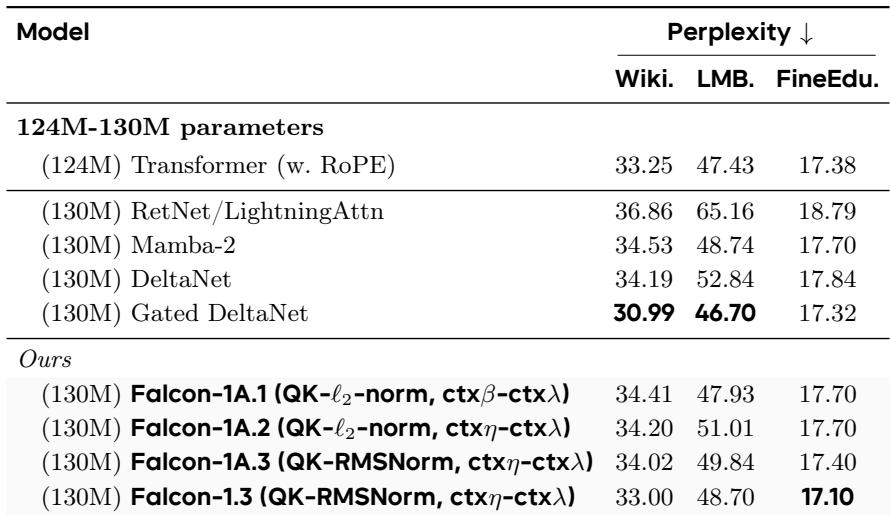
At 124M-130M parameters and a 50B-token budget, the proposed Falcon-1.3 model achieves the best FineWeb-Edu perplexity among all listed models, outperforming both the Transformer and recurrent baselines. Among recurrent baselines, Gated DeltaNet is the strongest, while Falcon-1A.3 leads the inner-product variants. The results show that the proposed aligned, normalized updates maintain competitive language modeling quality. Falcon-1.3 achieves the lowest FineWeb-Edu perplexity, surpassing all baselines including the Transformer and Gated DeltaNet. Gated DeltaNet is the best recurrent baseline on FineWeb-Edu, but still trails Falcon-1.3. Falcon-1A.3 is the best inner-product variant, with perplexity close to the top recurrent baseline. QK-RMSNorm improves FineWeb-Edu perplexity over QK-l2 normalization in the small scalar ablation.
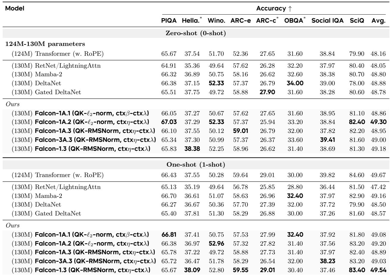
On the 124M-130M downstream evaluation, the proposed Falcon variants achieve competitive zero-shot and one-shot averages, with Falcon-1A.2 leading zero-shot and Falcon-1.3 leading one-shot among recurrent models. The results show no uniform win over baselines, but the aligned, normalized updates preserve language-model quality while enabling controlled arithmetic gains. Falcon-1A.2 achieves the best zero-shot average among listed models, while Falcon-1.3 has the best recurrent one-shot average. Among recurrent baselines, DeltaNet and Mamba-2 outperform RetNet/LightningAttn on the zero-shot average. The proposed variants do not uniformly beat baselines, but maintain competitive downstream accuracy across tasks.
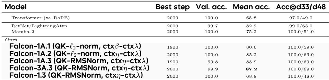
On variable-length multi-digit addition, the proposed Falcon variants generally match or exceed baseline models in validation accuracy, while showing stronger extrapolation to longer digit lengths. Among the listed models, Falcon-1A.3 achieves the highest mean accuracy and the best accuracy on the longest tested lengths, surpassing both the Transformer and recurrent baselines. Falcon-1A.3 attains the highest mean accuracy among all listed models, outperforming the Transformer and RetNet/LightningAttn. All Falcon variants reach near-perfect validation accuracy, with Falcon-1A.3 slightly lower at 99.8%. On the longest digit lengths, Falcon-1A.3 achieves the best accuracy, while the Transformer and Mamba-2 lag notably.
The evaluation covers language modeling, downstream tasks, and arithmetic reasoning. At 124M-130M parameters, Falcon-1.3 achieves the best FineWeb-Edu perplexity among all baselines, with Gated DeltaNet as the strongest recurrent competitor and Falcon-1A.3 leading inner-product variants. On downstream zero-shot and one-shot averages, Falcon variants remain competitive but do not uniformly outperform baselines, with Falcon-1A.2 leading zero-shot and Falcon-1.3 leading one-shot among recurrent models. In variable-length multi-digit addition, Falcon variants match or exceed baselines in validation accuracy and show stronger extrapolation to longer digit lengths, with Falcon-1A.3 achieving the highest mean accuracy and best performance on the longest tested lengths. Overall, the aligned, normalized updates preserve language-model quality while enabling controlled arithmetic gains.