Command Palette
Search for a command to run...
Machine Learning vs. Dynamic Models, Ai2's Latest Research: ACE2 Can Complete a 4-Month Seasonal Forecast in Just 2 Minutes

From farmland irrigation planning to cold wave disaster prevention and control, seasonal weather forecasts are crucial for disaster prevention and mitigation, agricultural production, and energy scheduling. For a long time, these forecasts relied on dynamic models based on physical equations. However, with the advancement of AI, machine learning models have now rivaled traditional models in key metrics, even achieving superior accuracy in some scenarios.
The core advantage of machine learning models is "autoregressive forecasting":Simulating short-term atmospheric evolution over a 1-6 hour period, feeding the forecast results into the model, generates high-precision multi-day forecasts. Some models can accurately forecast for weeks, and large-scale ensemble forecasts can also enhance the ability to predict the probability of extreme weather. However, significant bottlenecks exist: Forecasts exceeding several weeks are prone to reduced stability and loss of detail, making it difficult to meet seasonal timescale requirements. Furthermore, the physical mechanisms of the models are difficult to interpret, and the seasonal forecast sample size is small (only one independent sample per year). Using physical model simulation data to expand the training set also carries with it inherited errors.
It is in this technical context thatA research team consisting of the Met Office Exeter Hadley Centre, the University of Exeter, and the Allen Institute for Artificial Intelligence (Ai2) in the United States evaluated the previously developed machine learning weather model ACE2 and compared it with the dynamic model GloSea.The results show that ACE2 can maintain stability in long-term autoregressive forecasts and has preliminary potential for seasonal forecasts without complex ocean-air coupling, simply by learning atmospheric evolution from ERA5 historical data. This study confirms for the first time thatMachine learning models can generate highly skilled global seasonal forecasts, providing new directions for the development of short-term climate forecasting technology.
The relevant research results were published in npj Climate and Atmospheric Science under the title "Skilful global seasonal predictions from a machine learning weather model trained on reanalysis data."
Paper address:
Follow the official account and reply "ACE2" to get the complete PDF
More AI frontier papers:
Dataset: Multi-source data integration for seasonal forecast model evaluation
This study integrates multi-source data to support seasonal forecast model evaluation. The core data sources and processing methods are as follows:
Historical atmospheric basic data are taken from the ERA5 reanalysis dataset,To ensure the stability of sea surface temperature (SST) and sea ice conditions throughout the forecast period, the study applied a Gaussian rolling mean filter with a standard deviation of 10 days to each grid cell based on 6-hourly resolution atmospheric raw data to construct a climate background field that combines seasonal variation characteristics with boundary condition stability.
The monthly precipitation observation data are from the Global Precipitation Climatology Project (GPCP) v2.3 dataset.Provide an observational benchmark for verifying subsequent precipitation forecast results.
The traditional dynamical model data used for comparison were obtained from the GloSea operational ensemble forecast system (configured as GC3.2), using hindcast data initialized annually from 1993 to 2015. This system consists of 63 ensemble members, initialized in three batches (21 members each on October 25, November 1, and November 9 of each year). The ensemble spread is generated using a stochastic physics scheme. Its simulations have a forecast horizon of six months, with a resolution of approximately 0.5° for the atmosphere and 0.25° for the oceans. The model has 85 vertical levels for the atmosphere (extending to 85 km in the stratosphere) and 75 vertical levels for the oceans. It performs excellently for subseasonal to seasonal forecasts in tropical and mid-latitude regions, representing a leading dynamical model in this field.
To unify the comparison benchmark of forecast results,All ERA5 reanalysis data and GloSea model data in this study were converted to the native 1°×1° grid of ACE2 through bilinear interpolation, and only the precipitation data were interpolated to a 2.5°×2.5° grid.To accurately quantify key climate signals, the study defined and validated core climate indices. ENSO events were determined using the December-February (DJF) Ocean Niño Index (ONI), with a threshold of ±0.5 K. Eight El Niño winters and nine La Niña winters were identified. The NAO index is defined as the difference in mean sea level pressure between the north-south region (20°N-55°N and 55°N-90°N).
In the ensemble selection and forecast performance evaluation phase, this study selected members from a specific initialization time window to ensure comparability: ACE2 initialized members from October 28 to November 1 (n=20), and GloSea initialized members on November 1 (n=21). NAO values were aggregated into a 5-day climatological mean, and the climatological mean state was removed. The study calculated the ensemble mean error (RMSEₚ) and dispersion (based on σᵢₚ). Performance was evaluated from a signal-to-noise perspective using the predictable component ratio (RPC), with significance tested using a random resampling method.
Seasonal forecast implementation of the ACE2 model: combining data-driven and physical constraints
The ACE2 machine learning atmospheric model used in this study takes "combining data-driven and physical constraints" as its core design concept.Trained solely on ERA5 reanalysis atmospheric fields, the model accurately predicts atmospheric state evolution every six hours at a 1° grid resolution and maintains excellent stability in long-term autoregressive forecasts. This performance is due to three key design features: a spherical Fourier neural operator architecture that effectively captures atmospheric evolution patterns in spherical space; user-defined ocean and sea ice boundary conditions to accommodate diverse forecast scenarios; and constraints on key physical processes such as mass conservation, water vapor circulation, precipitation rate, and radiation flux to ensure physically consistent forecast results.
In seasonal-scale forecasts, ACE2 uses a lagged ensemble method to generate forecast results.During the period 1993–2015, the model initialized an ensemble member every six hours from October 25 to November 9 each year, generating a total of 64 members throughout the year. All initialization fields were derived from ERA5 reanalysis data to ensure the authenticity of the initial states. Forecasts were maintained from the initialization moment until mid-March of the following year, corresponding to a forecast timeframe of one to three months.
In terms of boundary condition processing, ACE2 uses continuous sea surface temperature (SST) and sea ice anomaly data.Based on the instantaneous anomaly of each grid cell at the time of initialization, combined with a 6-hour resolution climate state derived from ERA5 data, this anomaly is fixed throughout the forecast period. This strategy, unlike the time-varying boundary conditions used during training, helps reduce the interference caused by boundary fluctuations in seasonal forecasts. The climate state is based on 23 years of ERA5 data from 1994 to 2016, smoothed with a Gaussian filter with a standard deviation of 10 days. The SST boundary for any grid cell at time t is calculated using the formula. The sea ice concentration is treated in the same manner, and the result is strictly constrained to a reasonable range of 0–1.
In addition, the downward shortwave radiation flux from the top of the atmosphere and the global mean CO₂ concentration were modeled using the traditional dynamical model GloSea to ensure consistent boundary conditions for comparison. The sensitivity of ACE2 to these two boundary conditions requires further study.
To assess the sensitivity of these boundary conditions, the study conducted multiple controlled experiments. When using data from 1988–2022 to infer the climate state, the NAO correlation coefficient was 0.54; when using shortwave radiation flux from the previous year, the NAO correlation coefficient was 0.43; and when using CO₂ data from the previous year, the NAO correlation coefficient was 0.38. These results are consistent with a natural variability test (where the NAO correlation coefficient was 0.42 when initialization was delayed by 6 hours), indicating that ACE2 is insensitive to these boundary condition variations during the current seasonal forecasting mission, demonstrating good forecast stability.
ACE2 demonstrates excellent forecasting skills based on only 6 hours of observational evolution training
Multiple studies have confirmed that machine learning has not only promoted technological innovation in short-term weather forecasting, but also opened up new paths for the development of short-term climate prediction (seasonal scale).
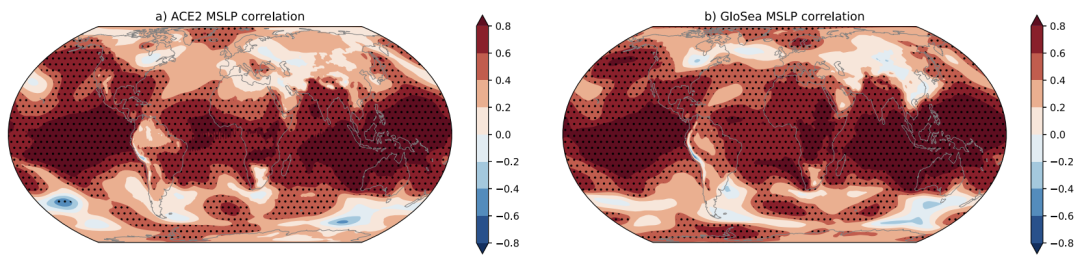
Over the 23-year evaluation period (1993–2015), as shown in the figure below, the ACE2 model exhibited highly similar skill distribution characteristics to the traditional dynamical model GloSea in seasonal forecasts with time horizons of 1–3 months, with particularly strong performance in mean sea level pressure (MSLP) forecasts. It is worth noting that ACE2's core design goal is to achieve stable climate simulations, and it was not specifically optimized for seasonal forecasts. Therefore, this cross-scenario performance consistency is more valuable for reference. Similar to GloSea, ACE2's MSLP forecast skill over Europe is relatively low, reflecting the common challenges of complex climate variability and forecasting difficulties in this region.
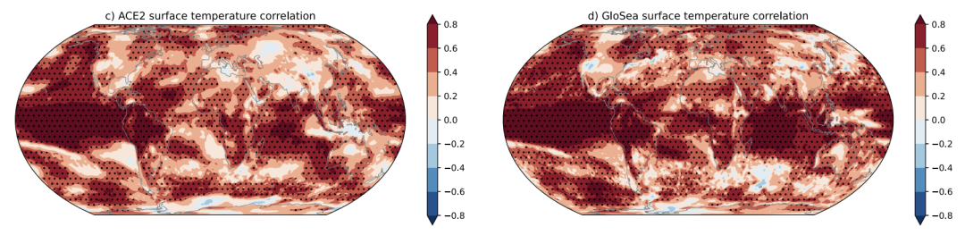
Quantitatively, ACE2's correlation coefficient is slightly lower than GloSea's in most regions. In terms of temperature forecasts, as shown in the figure below, ACE2 maintains effective forecasting capabilities over a wide range, covering South America, Africa, Australia, and parts of North America. Its skill distribution pattern is highly consistent with that of MSLP forecasts: ACE2's area-weighted average correlation coefficient for the temperate zone of the Northern Hemisphere is 0.41 (GloSea's is 0.45), while for the tropical regions, it is 0.68 and 0.77.
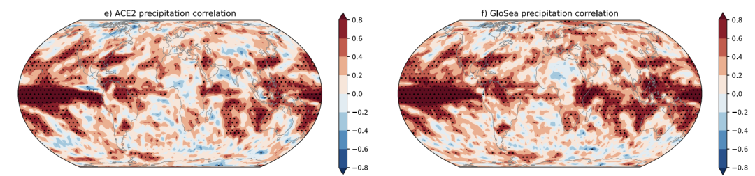
In precipitation forecasts, the overall skill of both models is relatively low. As shown in the figure below, the spatial distribution of ACE2's skill remains remarkably consistent with GloSea, particularly in the tropics, the Caribbean, and East Asia. This result further confirms ACE2's ability to forecast seasonal variability in multiple regions around the world.
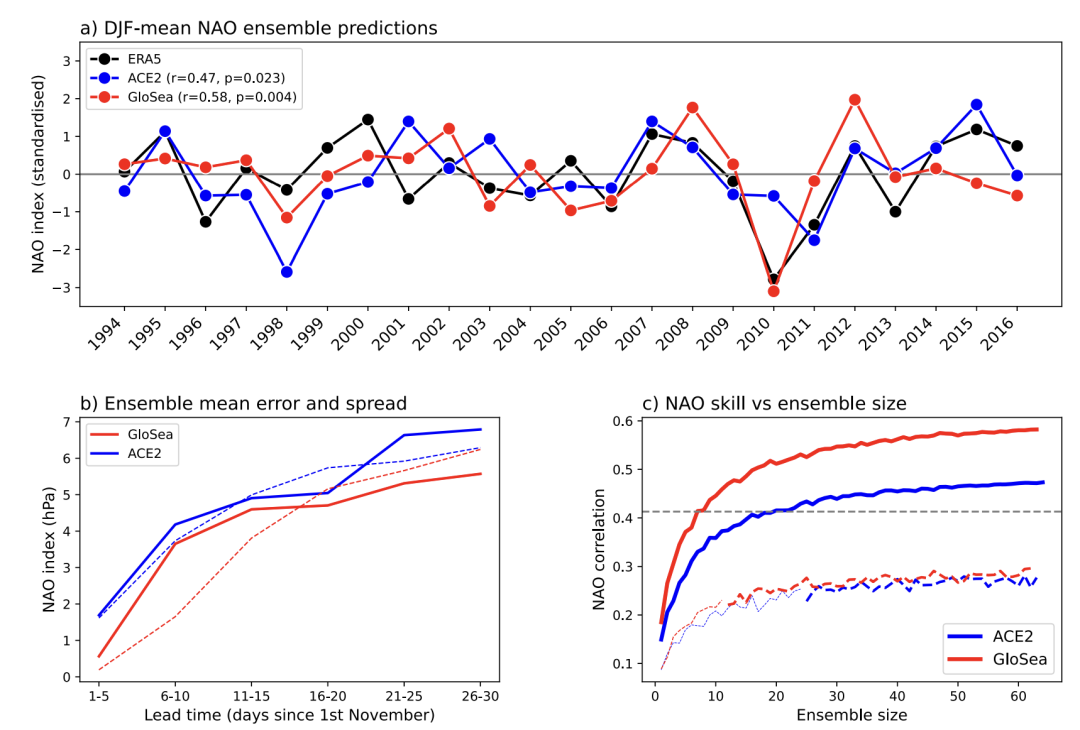
The two types of models also show significant complementarity in NAO forecasts. The correlation coefficient between ACE2 and GloSea's NAO forecasts was only 0.34 (p=0.11), but after ensemble averaging the two results, the correlation coefficient increased to 0.65 (p<0.01), making the accuracy comparable to GloSea's extended ensemble using 127 members. The evolution of the ensemble dispersion and mean error, as shown in the figure below, also shows a high degree of consistency between the two, further confirming the rationality of the ACE2 ensemble forecast.
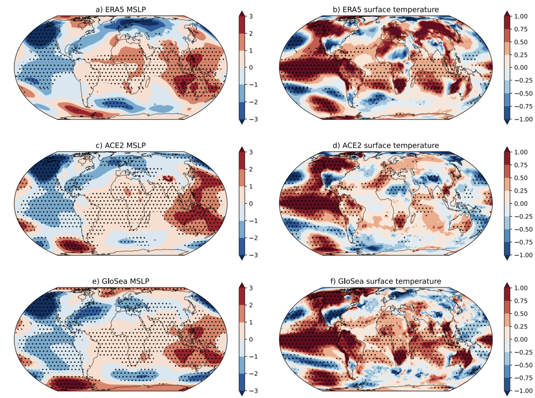
ACE2 also excels in capturing key climate modes, simulating the teleconnection of the El Niño-Southern Oscillation (ENSO). As shown in the figure below, by comparing the composite differences in climate fields between El Niño and La Niña years, we can see that the teleconnection patterns exhibited by ACE2 for two key variables, MSLP and surface temperature, are highly consistent with ERA5 reanalysis data and GloSea simulation results.It was confirmed that even with only 6-hour atmospheric evolution training, ACE2 can still accurately identify the interannual variability signals related to ENSO in multiple regions around the world.
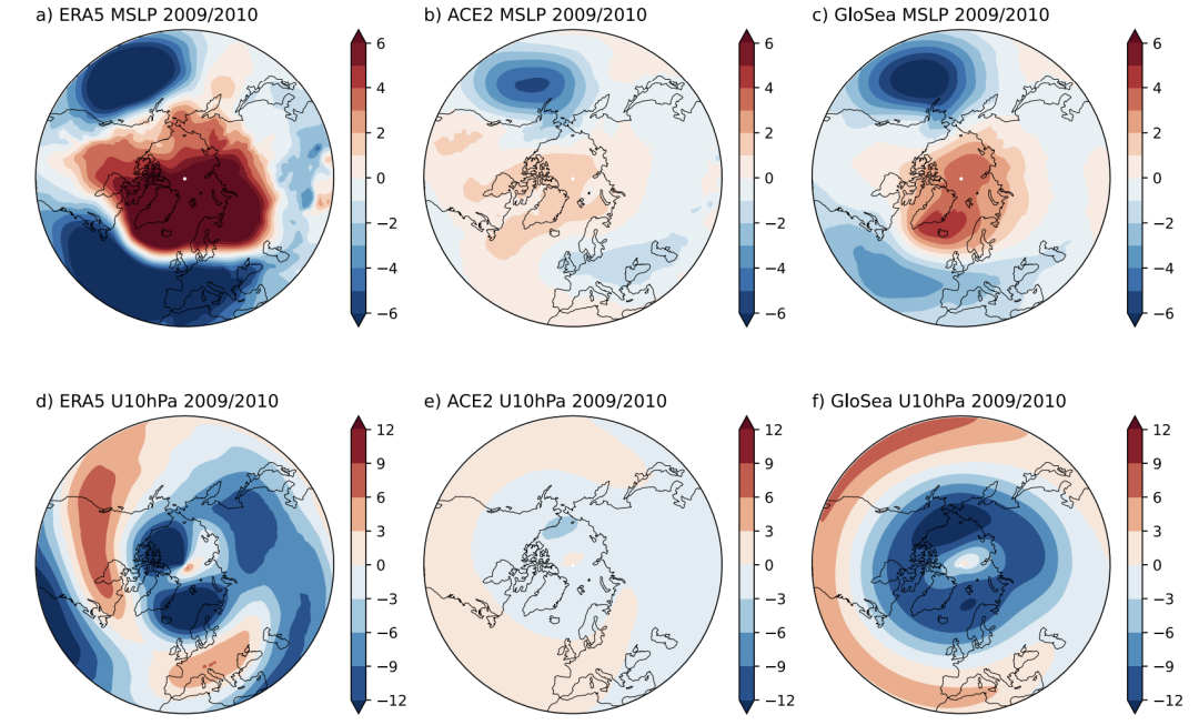
However, ACE2's limitations were evident in its forecasts of the extreme winter of 2009/2010: its ensemble mean did not accurately reproduce the negative NAO anomaly of the MSLP, simulating only slightly above-average Arctic pressure. Simulations of the stratospheric polar vortex were close to the climatological average, while both ERA5 and GloSea showed a significant weakening of the polar vortex. Regarding SSW forecasts, GloSea captured the enhancing effects of ENSO and the easterly QBO on SSW probability. ACE2 only exhibited stratospheric easterlies in the 39% member, with no difference in climatological occurrence from the 40%. Furthermore, its simulated SSW probabilities showed no statistical difference between El Niño years (45%), La Niña years (36%), and neutral years (41%), indicating that it did not fully capture the teleconnection between ENSO and the stratosphere.
The significant advantage of machine learning models is also reflected in computational efficiency. ACE2 completes a 4-month seasonal forecast in less than 2 minutes on a single NVIDIA A100 GPU.A single simulation of a traditional dynamic model would take several hours to run on a supercomputer. This efficiency advantage opens up more possibilities for technological innovation in seasonal forecasting.
In summary, the ACE2 series of forecast results fully demonstrate that machine learning methods are not only suitable for short-term weather forecasts, but can also provide new paths for technological breakthroughs and operational applications in short-term climate forecasts, providing important technical support for climate risk warnings in the context of global climate change.
Global academic and industrial collaboration: AI reshapes weather forecasting
In recent years, the rapid development of artificial intelligence technology is profoundly changing the field of weather forecasting, especially showing significant potential in seasonal and climate forecasting. Universities and research institutions continue to make breakthroughs in theoretical innovation. For example,The CERA machine learning framework developed by the Massachusetts Institute of Technology (MIT) provides a new path for climate prediction in the context of global warming.This framework does not rely on labeled data from a high greenhouse gas scenario. Instead, it combines controlled climate data with unlabeled warm climate inputs, effectively improving the model's generalization capabilities under unknown climate conditions. CERA not only captures the changing trends of key climate elements such as moisture transport and energy cycles, but also restores the vertical structure and meridional distribution of water vapor, demonstrating high accuracy in predicting the probability of extreme precipitation.
The business community is more focused on promoting technology implementation and efficiency improvement, and is committed to integrating machine learning models into actual business systems.The GraphCast model developed by Google DeepMind achieves minute-level generation of global 10-day weather forecasts based on graph neural networks.Many of its forecast indicators have surpassed the traditional numerical models of the European Centre for Medium-Range Weather Forecasts (ECMWF), providing important support for disaster emergency response.
Nvidia has launched FourCastNet in collaboration with the National Oceanic and Atmospheric Administration (NOAA) and other agencies.Relying on Fourier neural operators to achieve high-resolution global modeling, the prediction time of extreme weather is 12-24 hours earlier than traditional methods, which buys more response time for disaster prevention and mitigation.
Looking ahead, with the deepening of interdisciplinary collaboration, the improvement of high-quality multi-source meteorological datasets, and the continued evolution of the "physical constraints + data-driven" hybrid modeling framework, machine learning is expected to become the key core of the next generation of climate forecasting systems, providing more reliable scientific support for responding to climate change, ensuring agricultural production, and enhancing disaster prevention capabilities.
Reference Links:
1.https://mp.weixin.qq.com/s/Q5zJUwpeT88DvojgAA1afA
2.https://mp.weixin.qq.com/s/ZqlLWpoDSdFo82Qw44Sb3A