Command Palette
Search for a command to run...
Das Hören des Rauschens: Blind-Denoising mit Gibbs-Diffusion
Das Hören des Rauschens: Blind-Denoising mit Gibbs-Diffusion
David Heurtel-Depeiges Charles C. Margossian Ruben Ohana Bruno Régaldo-Saint Blancard
Zusammenfassung
In den letzten Jahren sind Rauschunterdrückungsprobleme eng mit der Entwicklung tiefer generativer Modelle verflochten. Insbesondere werden Diffusionsmodelle wie Rauschunterdrückungsmodelle trainiert, und die Verteilung, die sie modellieren, entspricht im bayesschen Bild den Rauschpriori. Allerdings erfordert die Rauschunterdrückung mittels posteriorer Sampling basierend auf Diffusionsmodellen, dass die Rauschstärke und die Kovarianz bekannt sind, was eine blinde Rauschunterdrückung unmöglich macht. Wir überwinden diese Einschränkung durch die Einführung von Gibbs Diffusion (GDiff), einer allgemeinen Methodologie zur posterioren Stichprobenerzeugung sowohl des Signals als auch der Rauschparameter. Unter der Annahme einer beliebigen parametrischen Gaußschen Rauschverteilung entwickeln wir einen Gibbs-Algorithmus, der abwechselnd Stichproben aus einem bedingten Diffusionsmodell zieht, das darauf trainiert ist, den Signalprior auf die Familie der Rauschverteilungen abzubilden, und aus einem Monte-Carlo-Sampler zur Schätzung der Rauschparameter. Unsere theoretische Analyse hebt mögliche Fallstricke hervor, leitet eine diagnostische Nutzung an und quantifiziert Fehler in der stationären Verteilung des Gibbs-Algorithmus, die durch die Approximation des Diffusionsmodells verursacht werden. Wir demonstrieren unsere Methode an zwei Anwendungen: 1) blinder Rauschunterdrückung natürlicher Bilder mit farbigem Rauschen unbekannter Amplitude und Spektralindex sowie 2) einem Problem der Kosmologie, nämlich der Analyse von kosmischen Mikrowellenhintergrund-Daten, bei dem die bayessche Inferenz der „Rausch“-Parameter der Einschränkung von Modellen zur Entwicklung des Universums entspricht.
One-sentence Summary
The authors, affiliated with institutions including the University of Paris-Saclay and the French National Centre for Scientific Research, propose Gibbs Diffusion (GDiff), a novel framework enabling blind posterior sampling of both signals and unknown noise parameters in diffusion models by alternating between a conditional diffusion sampler and a Monte Carlo noise parameter estimator. Unlike prior methods requiring known noise statistics, GDiff leverages parametric Gaussian noise assumptions and a Gibbs iterative scheme to jointly infer signals and noise characteristics, demonstrating success in blind image denoising with colored noise and cosmological inference for cosmic microwave background data, where it enables Bayesian constraints on early-universe models.
Key Contributions
- The paper addresses blind denoising in a Bayesian framework, where both the signal and unknown noise parameters (e.g., amplitude and spectral index of colored noise) must be inferred from observations, overcoming the limitation of standard diffusion models that require known noise covariance.
- It introduces Gibbs Diffusion (GDiff), a novel Gibbs sampling method that alternates between a conditional diffusion model trained to map the signal prior to noise distributions and a Monte Carlo sampler for noise parameters, enabling joint posterior inference over both signal and noise.
- The method is validated on natural image denoising with unknown colored noise and on cosmological analysis of cosmic microwave background data, demonstrating state-of-the-art performance and providing theoretical guarantees on the stationary distribution and error propagation.
Introduction
Denoising has evolved significantly with deep generative models, particularly diffusion models, which excel at learning complex signal priors and enabling posterior sampling. However, existing methods typically require known noise characteristics—such as amplitude and covariance—limiting their applicability to blind denoising scenarios where noise parameters are unknown. This constraint hinders critical applications in fields like medical imaging, astronomy, and cosmology, where accurate noise modeling is essential for reliable inference. The authors introduce Gibbs Diffusion (GDiff), a novel framework that jointly samples the signal and unknown noise parameters by combining a diffusion model trained to map the signal prior to a family of noise distributions with a Monte Carlo sampler for noise parameter inference. Their approach enables blind denoising under arbitrary parametric Gaussian noise, provides theoretical guarantees on the existence of a stationary distribution, and quantifies error propagation. The method is demonstrated on natural image denoising with colored noise and cosmological analysis of cosmic microwave background data, where noise parameters correspond to fundamental cosmological models.
Dataset
- The dataset comprises two primary components: natural images from ImageNet 2012 and simulated cosmological data for dust emission and CMB anisotropies.
- For natural images, the authors use the full ImageNet 2012 training set of 1,281,167 images, resized to 3 × 256 × 256 and center-cropped. Images are augmented with random horizontal flips and normalized to the [0, 1] range.
- The cosmological dataset is derived from the CATS database (Burkhart et al., 2020), using turbulent hydrodynamic simulations of the diffuse interstellar medium. Dust emission maps are constructed as proxies for gas column density, resulting in 991 simulated maps of size 256 × 256. Ten percent of these maps are reserved for validation.
- CMB maps are generated by sampling Gaussian random fields on the sphere with covariance matrices Σφ derived from cosmological parameters φ, using CAMB for power spectrum computation and pixell for projection onto 256 × 256 patches with 8' pixel resolution. The effective sky coverage is approximately 34 × 34 deg².
- Training examples are created by combining dust maps with CMB realizations, where cosmological parameters (H₀ and ω_b) are sampled from a prior distribution p(φ). A differentiable neural emulator approximates the mapping φ → Σφ to enable efficient training and gradient computation for HMC.
- The diffusion model is trained on ImageNet data for 100 epochs using 8 H100 GPUs with a batch size of 128 per GPU, employing AdamW optimizer with no learning rate schedule and weight decay set to 0.
- For the cosmological application, training spans 100,000 epochs on a single A100 80GB GPU with a batch size of 64, using AdamW with an inverse square root learning rate scheduler and warm-up. Training is continued beyond loss plateauing to improve model precision, as validated by simulation-based calibration.
Method
The authors leverage diffusion models to address blind denoising within a Bayesian framework, formulating the problem as posterior sampling of the joint distribution p(x,ϕ∣y). The core of their method, named GDiff, is a Gibbs sampling algorithm that iteratively constructs a Markov chain by alternating between two conditional sampling steps. The first step involves sampling the signal x given the observation y and the noise parameters ϕ, while the second step involves sampling the noise parameters ϕ given the observation y and the current signal estimate x. This iterative process aims to produce samples from the target joint posterior distribution after a sufficient number of iterations.
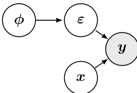
The graphical model in the figure above illustrates the generative process underlying the blind denoising problem. It shows that the observed data y is generated from the true signal x and the noise parameters ϕ, which in turn generate the noise ε. The goal is to infer the latent variables x and ϕ from the observation y, which is a classic Bayesian inference problem. The GDiff algorithm directly targets this inference by constructing a Markov chain that explores the joint posterior distribution p(x,ϕ∣y).
The first sampling step, p(x∣y,ϕ), is addressed using a diffusion model. The authors show that a diffusion model can be trained to both define a prior p(x) and provide an efficient means to sample the posterior distribution p(x∣y,ϕ). This is achieved by training the model to reverse a forward stochastic process, which gradually adds noise to the data. The forward process is defined by a stochastic differential equation (SDE) that models the noising of the signal x over time. The reverse SDE, which the diffusion model learns to approximate, allows for the generation of samples from the posterior distribution. In practice, the diffusion model is conditioned on the noise parameters ϕ, which are provided as an input to the score network, enabling the model to handle a range of noise configurations consistent with the prior p(ϕ).
The second sampling step, p(ϕ∣y,x), is equivalent to sampling p(ϕ∣ε) where ε=y−x is the residual noise. This step is performed using a Hamiltonian Monte Carlo (HMC) sampler. The HMC algorithm requires the ability to efficiently evaluate and differentiate the log posterior distribution logp(ϕ∣ε), which is composed of the log prior logp(ϕ) and the log likelihood logp(ε∣ϕ). For the Gaussian noise model considered, the log likelihood has a closed-form expression, making it straightforward to implement. The HMC sampler constructs a Markov chain that yields samples from the target distribution p(ϕ∣ε) once the stationary regime is reached.
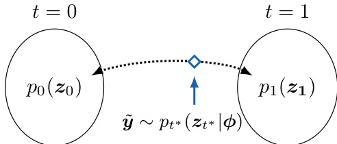
The figure above illustrates the reverse SDE process, which is central to the diffusion model's ability to sample from the posterior. It shows the transition from the initial distribution p0(z0), which corresponds to the prior p(x), to the final distribution p1(z1), which is a highly noisy distribution. The reverse process, starting from a point y~ at time t=1, flows backward in time to generate samples from the posterior distribution p(x∣y,ϕ). This process is defined by a reverse SDE that depends on the score function of the current distribution, which the diffusion model learns to approximate. The algorithm iterates between these two steps, using the diffusion model to sample the signal and the HMC sampler to sample the noise parameters, to generate samples from the joint posterior distribution.
Experiment
- Evaluated on blind denoising of natural images with colored noise and cosmological inference from CMB data with Galactic foregrounds, demonstrating effective convergence of the Gibbs sampler in both settings.
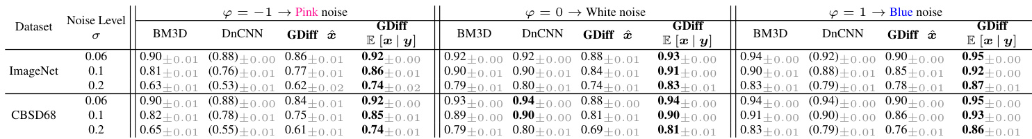
- On the ImageNet-based denoising task, GDiff achieved SSIM of 0.896 (posterior mean) and 0.882 (posterior sample), outperforming DnCNN (trained on white noise) and matching BM3D (non-blind) despite being blind.
- On CMB data, the method successfully inferred noise parameters and recovered posterior distributions, though slight bias was observed due to diffusion model approximation errors.
- Guidance-based methods (DPS, II-GDM) failed due to numerical instabilities from high condition number (∼6×10⁵) of noise covariance, leading to poor posterior estimation and non-convergence in Gibbs sampling.
- Effective inference required time-dependent regularization, but even then, large-scale structures were poorly recovered, highlighting limitations of existing guidance methods in high-dynamic-range inverse problems.
Results show that GDiff achieves competitive image quality compared to BM3D and DnCNN across different noise types and levels, with SSIM values close to or exceeding those of the non-blind BM3D method. The method performs consistently well in both blind denoising and parameter estimation, as evidenced by stable posterior sampling metrics and effective recovery of noise-free images across various noise conditions.
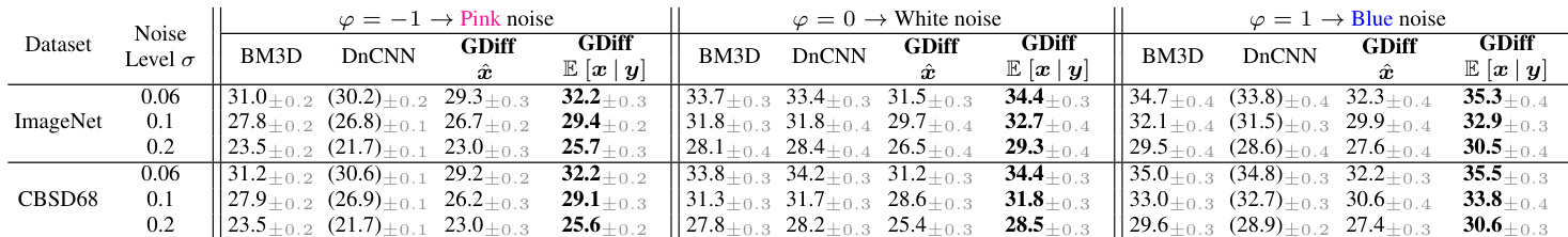
Results show that GDiff achieves competitive or superior performance compared to BM3D and DnCNN across different noise types and levels, with the best results observed under white noise conditions. The method demonstrates robustness in blind denoising, producing high-quality reconstructions and accurate posterior estimates, though performance varies depending on the noise model and dataset.