Command Palette
Search for a command to run...
GROMACS 入門チュートリアル: 水中のリゾチーム
「水中のリゾチーム」を例に分子動力学シミュレーションを行う
チュートリアルの紹介
このチュートリアルは、GROMACS ソフトウェアを使用した分子動力学シミュレーションの入門チュートリアルです。 水中のリゾチーム 例として、水中のタンパク質の典型的な分子動力学シミュレーションを準備して実行する方法を学びます。
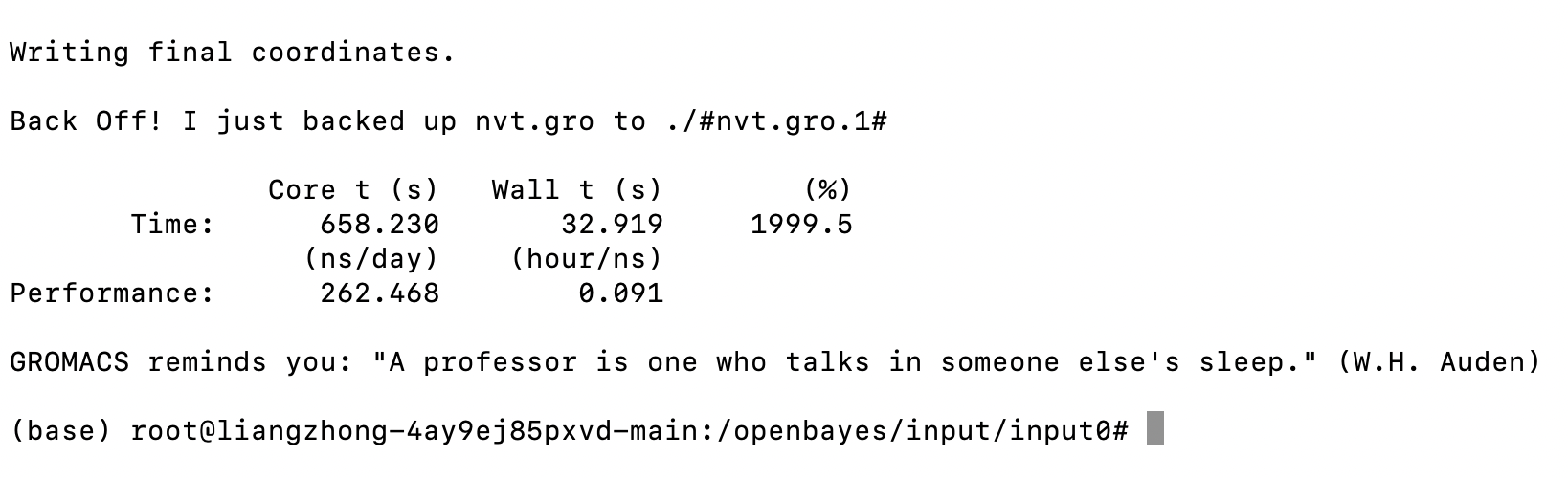
OpenBayes プラットフォーム上の NVIDIA RTX 4090 グラフィックス カードで構成された GROMACS の GPU バージョンを使用すると、GPU 並列コンピューティング後のコンピューティング効率が大幅に向上し、速度は 255ns/日に達します。速度性能は以下の通りです。
            Core t (s)   Wall t (s)        (%)
Time:     3972.923      198.659     1999.9
                   (ns/day)    (hour/ns)
Performance:      255.471        0.094
GROMACS の概要
GROMACS (GRoningen MAchine for Chemical Simulations) は、分子動力学シミュレーション用の高性能ソフトウェア パッケージで、主にさまざまな条件下での生体分子 (タンパク質、脂質、核酸など) の運動挙動をモデル化およびシミュレーションするために使用されます。元々はオランダのフローニンゲン大学で開発されたもので、分子動力学の分野で最も一般的に使用されているオープンソース ツールの 1 つになりました。
GROMACSの主な特長
1. 高性能:
• GROMACS は並列コンピューティング用に高度に最適化されており、最新のマルチコア CPU および GPU システムで効率的に実行できます。
• マルチスレッドおよび分散コンピューティングのための OpenMP および MPI をサポートします。
2. 幅広い用途:
• 小さな分子から大きなタンパク質複合体までの挙動をモデル化するために使用できます。
• 生体分子、ポリマー、無機化合物、その他の化学システムの研究をサポートします。
3. 柔軟性:
• 前処理 (トポロジー生成、溶媒和など) および後処理 (軌道解析、エネルギー計算など) のための豊富なツールを提供します。
• AMBER、CHARMM、GROMOS などの複数の力場をサポートします。
4. 使いやすさ:
• GROMACS には、使いやすいコマンド ライン インターフェイスが含まれています。
• 初心者と上級ユーザーの両方に適した詳細なドキュメントとチュートリアルが提供されています。
5. オープンソースで拡張可能:
• オープン ソース ライセンスにより、ユーザーは特定のニーズに合わせて GROMACS を変更および拡張できます。
• 活発なユーザー コミュニティと開発チームを擁します。
GROMACS の一般的な使用プロセス
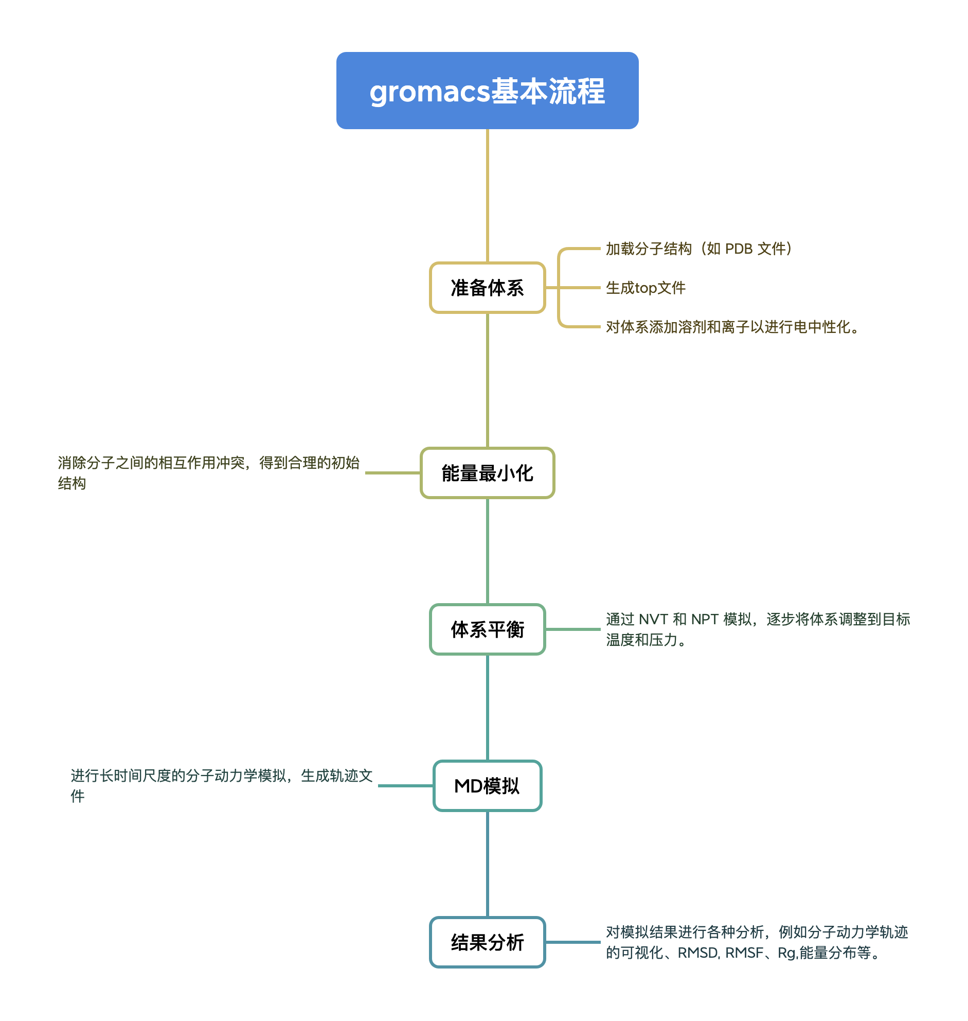
ステップの実行
まず、pdb タンパク質ファイルと md 計算ファイルを設定する必要があります。その後、さまざまな前処理を経て、最終的に 10ns のシミュレーションを実行して結果を解析します。以下、ステップバイステップで説明します。
1.GROMACSを起動する
首先登录平台:https://openbayes.com/
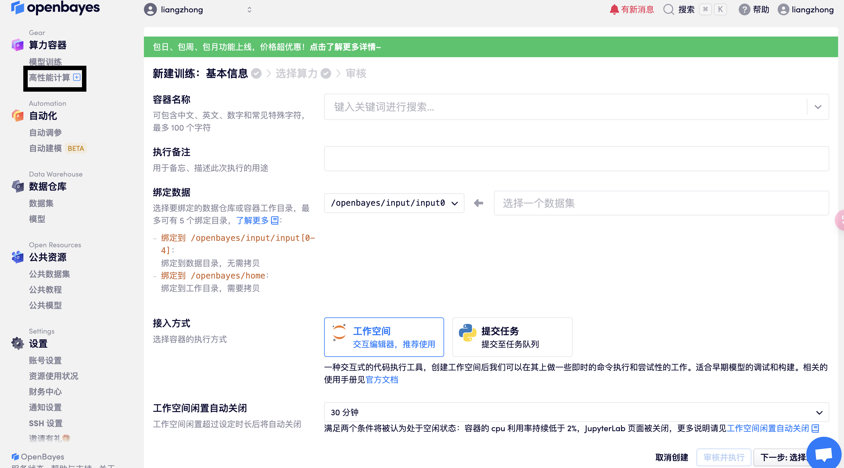
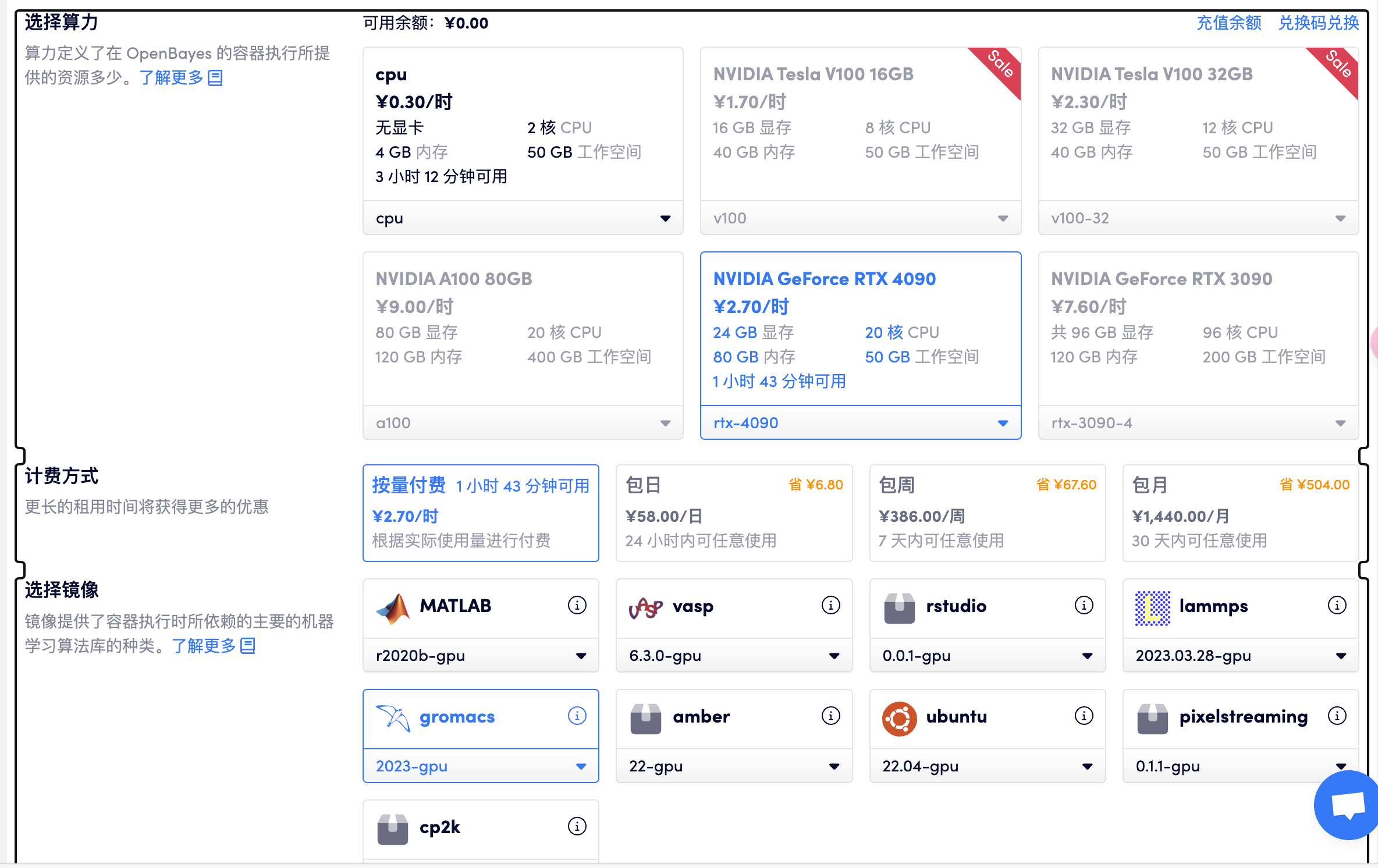
选择「高性能计算」> 创建新容器> 选择算力 RTX 4090> 选择 gromacs GPU
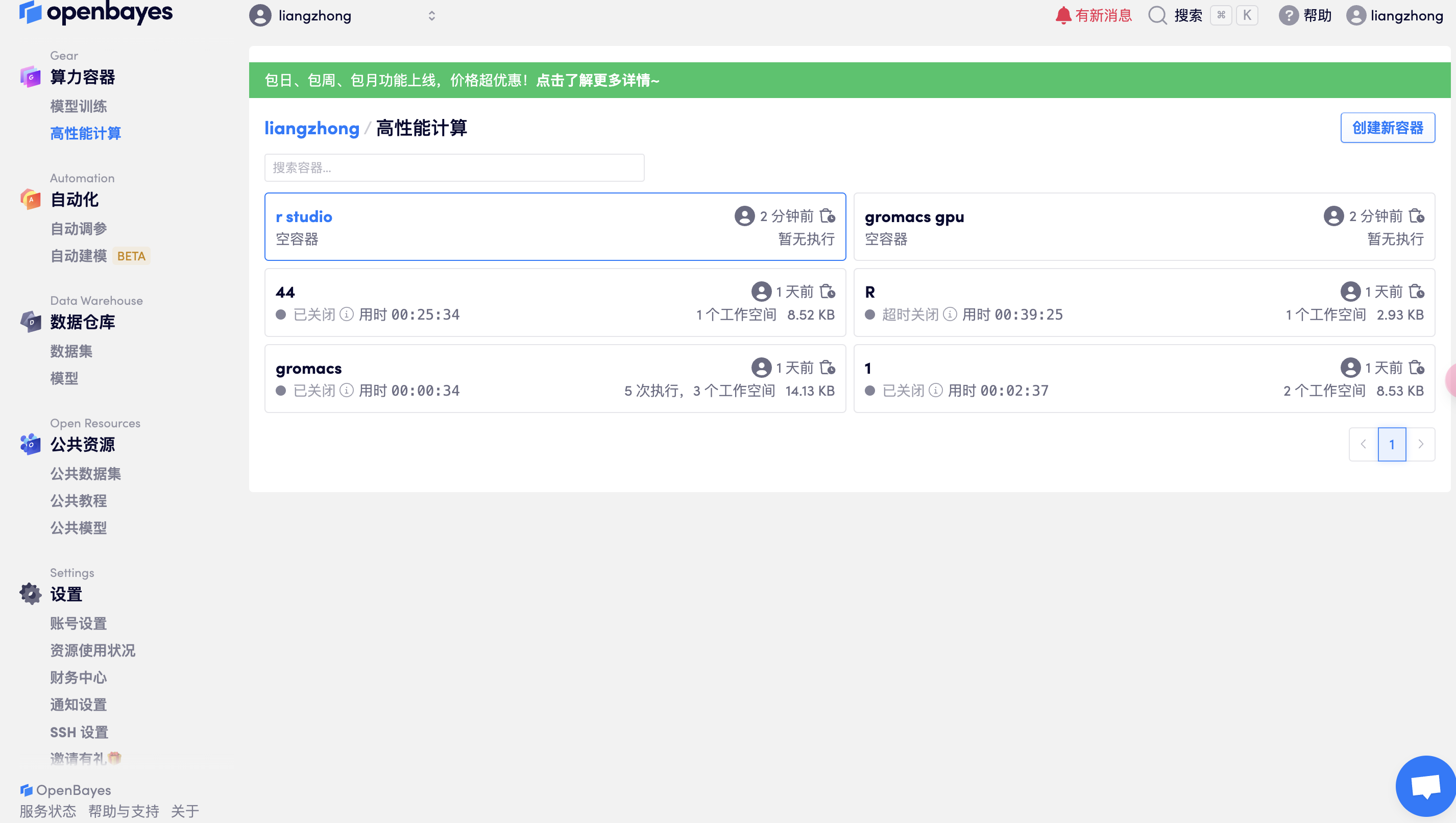
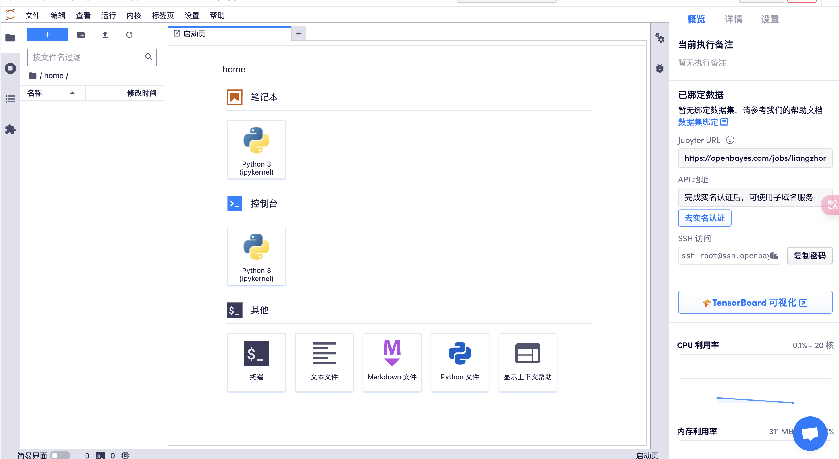
打开工作空间
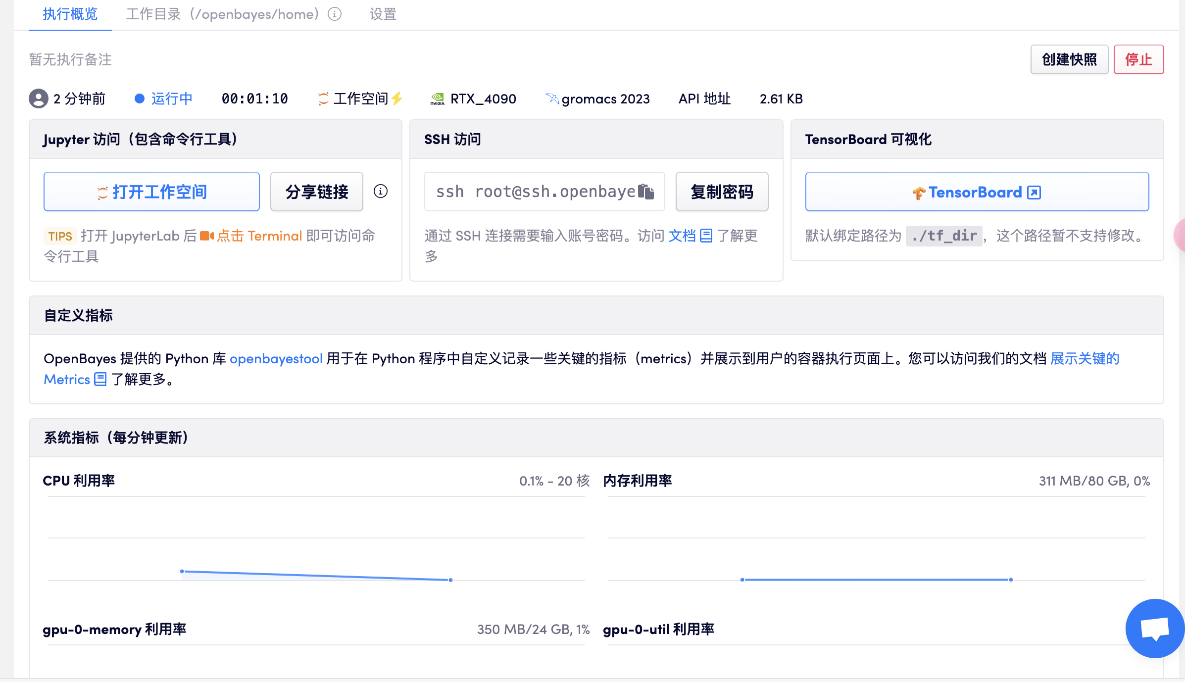
打开终端
或者采用 SSH 控制服务器:

在 X-shell 或者 mac unix 终端,输入:ssh -p 32699  [email protected],再输入密码即可(如下所示)↓
liangzhongzhongzhong@lzr ~ % ssh -p 32699  [email protected]
The authenticity of host '[ssh.openbayes.com]:32699 ([101.237.34.75]:32699)' can't be established.
ED25519 key fingerprint is SHA256:uwPyhP/EYoW49Ez4rvAuaf19czwis2rdS4pImsR0NH8.
This key is not known by any other names.
Are you sure you want to continue connecting (yes/no/[fingerprint])? yes
Warning: Permanently added '[ssh.openbayes.com]:32699' (ED25519) to the list of known hosts.
[email protected]'s password:
OpenBayes

目录说明

- /openbayes/home 工作空间内的数据保存地址,容器停止后,该目录中的内容不会被删除
- /openbayes/input/input0 - /openbayes/input/input4 为数据目录,不会占用工作空间的存储容量,最多支持同时绑定 5 个

⚠️  其他目录下的内容在容器关闭后会被自动删除!更多信息请访问 https://openbayes.com/docs/concepts
⚠️  禁止挖矿,一经发现将立即封号恕不退款

(base) root@liangzhong-4ay9ej85pxvd-main:/openbayes/home# ls
(base) root@liangzhong-4ay9ej85pxvd-main:/openbayes# l(base) root@liangzhong-4ay9ej85pxvd-main:/openbayes# lhome  input  请将文件存在 home 目录下, 当前文件夹下的文件不会被保存.txt
(base) root@liangzhong-4ay9ej85pxvd-main:/openbayes# ls(base) root@liangzhong-4ay9ej85pxvd-main:/openbaye
(base) root@liangzhong-4ay9ej85pxvd-main:/openbayes/input# cd input0
(base) root@liangzhong-4ay9ej85pxvd-main:/openbayes/input/input0# ls
'#nvt.log.1#'    '#topol.top.2#'    1AKI_processed.gro   1aki.pdb   em.log   ions.mdp   mdout.mdp   nvt.cpt   nvt.log   nvt.trr         topol.top
'#nvt.log.2#'     1AKI_clean.pdb    1AKI_solv.gro        em.edr     em.tpr   ions.tpr   minim.mdp   nvt.edr   nvt.mdp   posre.itp
'#topol.top.1#'   1AKI_newbox.gro   1AKI_solv_ions.gro   em.gro     em.trr   md.mdp     npt.mdp     nvt.gro   nvt.tpr   potential.xvg
(base) root@liangzhong-4ay9ej85pxvd-main:/openbayes/input/input0#

调用 GROMACS,设置临时环境变量
export PATH=/data/app/gromacs/bin:$PATH
(base) root@liangzhong-4ay9ej85pxvd-main:/openbayes/home# gmx_mpi -h
                        :-) GROMACS - gmx_mpi, 2023 (-:

Executable:   /data/app/gromacs/bin/gmx_mpi
Data prefix:  /data/app/gromacs
Working dir:  /output
Command line:
  gmx_mpi -h

SYNOPSIS

gmx [-[no]h] [-[no]quiet] [-[no]version] [-[no]copyright] [-nice <int>]
    [-[no]backup]

OPTIONS

Other options:

 -[no]h                     (no)
           Print help and quit
 -[no]quiet                 (no)
           Do not print common startup info or quotes
 -[no]version               (no)
           Print extended version information and quit
 -[no]copyright             (no)
           Print copyright information on startup
 -nice   <int>              (19)
           Set the nicelevel (default depends on command)
 -[no]backup                (yes)
           Write backups if output files exist

Additional help is available on the following topics:
    commands    List of available commands
    selections  Selection syntax and usage
To access the help, use 'gmx help <topic>'.
For help on a command, use 'gmx help <command>'.

GROMACS reminds you: "All You Need is Greed" (Aztec Camera)
2. 書類の準備
チュートリアルを実行する前に、次の 6 つのファイルを準備する必要があります: 1aki.pdb、ions.mdp、md.mdp、minim.mdp、npt.mdp、nvt.mdp
これらのファイルは直接ダウンロードすることも、次のように作成することもできます。
たとえば、1AKI.pdb タンパク質ファイルは次から取得できます。 RCSB Web サイトは 1AKI.pdb を取得します。このチュートリアルでは、vim テキスト エディターを使用してコードをコピーすることで、他のファイルが作成されています。
RCSB データベースの紹介:
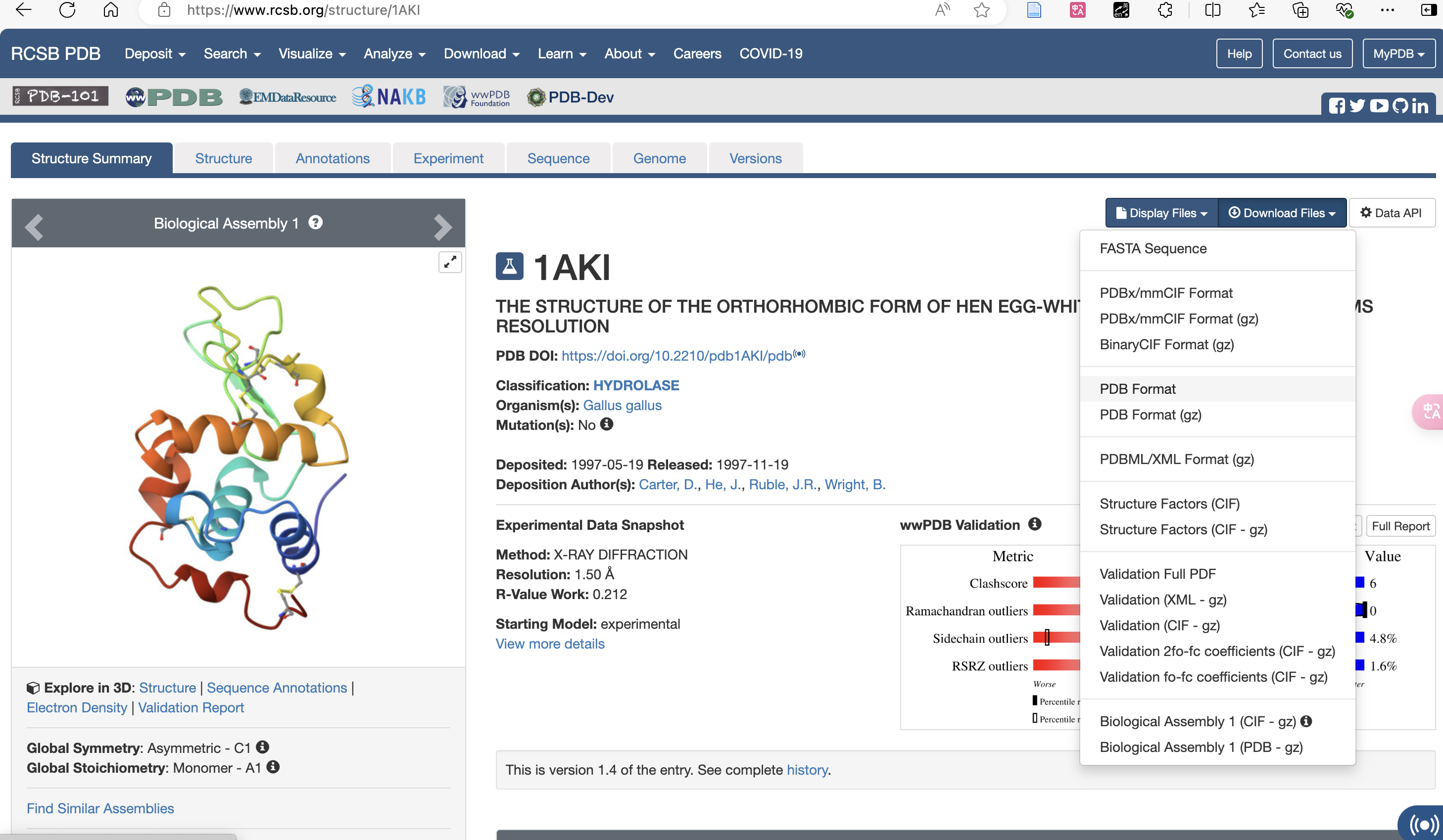
ダウンロード pdb フォーマット形式:
作業ディレクトリにアップロードする
(base) root@liangzhong-4ay9ej85pxvd-main:/input0# ls
1aki.pdb
#查看上传成功
vim ions.mdp
#准备 mdp 文件,输入命令后复制一下内容,按 i 进入插入模式开始编辑。
#编辑完成后,按 Esc 键退出插入模式,输入 :wq 保存并退出。
; ions.mdp - used as input into grompp to generate ions.tpr
; Parameters describing what to do, when to stop and what to save
integrator  = steep         ; Algorithm (steep = steepest descent minimization)
emtol       = 1000.0        ; Stop minimization when the maximum force < 1000.0 kJ/mol/nm
emstep      = 0.01          ; Minimization step size
nsteps      = 50000         ; Maximum number of (minimization) steps to perform

; Parameters describing how to find the neighbors of each atom and how to calculate the interactions
nstlist         = 1         ; Frequency to update the neighbor list and long range forces
cutoff-scheme	= Verlet    ; Buffered neighbor searching
ns_type         = grid      ; Method to determine neighbor list (simple, grid)
coulombtype     = cutoff    ; Treatment of long range electrostatic interactions
rcoulomb        = 1.0       ; Short-range electrostatic cut-off
rvdw            = 1.0       ; Short-range Van der Waals cut-off
pbc             = xyz       ; Periodic Boundary Conditions in all 3 dimensions
vim minim.mdp

; minim.mdp - used as input into grompp to generate em.tpr
; Parameters describing what to do, when to stop and what to save
integrator  = steep         ; Algorithm (steep = steepest descent minimization)
emtol       = 1000.0        ; Stop minimization when the maximum force < 1000.0 kJ/mol/nm
emstep      = 0.01          ; Minimization step size
nsteps      = 50000         ; Maximum number of (minimization) steps to perform

; Parameters describing how to find the neighbors of each atom and how to calculate the interactions
nstlist         = 1         ; Frequency to update the neighbor list and long range forces
cutoff-scheme   = Verlet    ; Buffered neighbor searching
ns_type         = grid      ; Method to determine neighbor list (simple, grid)
coulombtype     = PME       ; Treatment of long range electrostatic interactions
rcoulomb        = 1.0       ; Short-range electrostatic cut-off
rvdw            = 1.0       ; Short-range Van der Waals cut-off
pbc             = xyz       ; Periodic Boundary Conditions in all 3 dimensions
vim nvt.mdp

title                   = OPLS Lysozyme NVT equilibration
define                  = -DPOSRES  ; position restrain the protein
; Run parameters
integrator              = md        ; leap-frog integrator
nsteps                  = 50000     ; 2 * 50000 = 100 ps
dt                      = 0.002     ; 2 fs
; Output control
nstxout                 = 500       ; save coordinates every 1.0 ps
nstvout                 = 500       ; save velocities every 1.0 ps
nstenergy               = 500       ; save energies every 1.0 ps
nstlog                  = 500       ; update log file every 1.0 ps
; Bond parameters
continuation            = no        ; first dynamics run
constraint_algorithm    = lincs     ; holonomic constraints
constraints             = h-bonds   ; bonds involving H are constrained
lincs_iter              = 1         ; accuracy of LINCS
lincs_order             = 4         ; also related to accuracy
; Nonbonded settings
cutoff-scheme           = Verlet    ; Buffered neighbor searching
ns_type                 = grid      ; search neighboring grid cells
nstlist                 = 10        ; 20 fs, largely irrelevant with Verlet
rcoulomb                = 1.0       ; short-range electrostatic cutoff (in nm)
rvdw                    = 1.0       ; short-range van der Waals cutoff (in nm)
DispCorr                = EnerPres  ; account for cut-off vdW scheme
; Electrostatics
coulombtype             = PME       ; Particle Mesh Ewald for long-range electrostatics
pme_order               = 4         ; cubic interpolation
fourierspacing          = 0.16      ; grid spacing for FFT
; Temperature coupling is on
tcoupl                  = V-rescale             ; modified Berendsen thermostat
tc-grps                 = Protein Non-Protein   ; two coupling groups - more accurate
tau_t                   = 0.1     0.1           ; time constant, in ps
ref_t                   = 300     300           ; reference temperature, one for each group, in K
; Pressure coupling is off
pcoupl                  = no        ; no pressure coupling in NVT
; Periodic boundary conditions
pbc                     = xyz       ; 3-D PBC
; Velocity generation
gen_vel                 = yes       ; assign velocities from Maxwell distribution
gen_temp                = 300       ; temperature for Maxwell distribution
gen_seed                = -1        ; generate a random seed
vim npt.mdp

title                   = OPLS Lysozyme NPT equilibration
define                  = -DPOSRES  ; position restrain the protein
; Run parameters
integrator              = md        ; leap-frog integrator
nsteps                  = 50000     ; 2 * 50000 = 100 ps
dt                      = 0.002     ; 2 fs
; Output control
nstxout                 = 500       ; save coordinates every 1.0 ps
nstvout                 = 500       ; save velocities every 1.0 ps
nstenergy               = 500       ; save energies every 1.0 ps
nstlog                  = 500       ; update log file every 1.0 ps
; Bond parameters
continuation            = yes       ; Restarting after NVT
constraint_algorithm    = lincs     ; holonomic constraints
constraints             = h-bonds   ; bonds involving H are constrained
lincs_iter              = 1         ; accuracy of LINCS
lincs_order             = 4         ; also related to accuracy
; Nonbonded settings
cutoff-scheme           = Verlet    ; Buffered neighbor searching
ns_type                 = grid      ; search neighboring grid cells
nstlist                 = 10        ; 20 fs, largely irrelevant with Verlet scheme
rcoulomb                = 1.0       ; short-range electrostatic cutoff (in nm)
rvdw                    = 1.0       ; short-range van der Waals cutoff (in nm)
DispCorr                = EnerPres  ; account for cut-off vdW scheme
; Electrostatics
coulombtype             = PME       ; Particle Mesh Ewald for long-range electrostatics
pme_order               = 4         ; cubic interpolation
fourierspacing          = 0.16      ; grid spacing for FFT
; Temperature coupling is on
tcoupl                  = V-rescale             ; modified Berendsen thermostat
tc-grps                 = Protein Non-Protein   ; two coupling groups - more accurate
tau_t                   = 0.1     0.1           ; time constant, in ps
ref_t                   = 300     300           ; reference temperature, one for each group, in K
; Pressure coupling is on
pcoupl                  = Parrinello-Rahman     ; Pressure coupling on in NPT
pcoupltype              = isotropic             ; uniform scaling of box vectors
tau_p                   = 2.0                   ; time constant, in ps
ref_p                   = 1.0                   ; reference pressure, in bar
compressibility         = 4.5e-5                ; isothermal compressibility of water, bar^-1
refcoord_scaling        = com
; Periodic boundary conditions
pbc                     = xyz       ; 3-D PBC
; Velocity generation
gen_vel                 = no        ; Velocity generation is off
vim md.md

title                   = OPLS Lysozyme NPT equilibration
; Run parameters
integrator              = md        ; leap-frog integrator
nsteps                  = 500000    ; 2 * 500000 = 1000 ps (1 ns)
dt                      = 0.002     ; 2 fs
; Output control
nstxout                 = 0         ; suppress bulky .trr file by specifying
nstvout                 = 0         ; 0 for output frequency of nstxout,
nstfout                 = 0         ; nstvout, and nstfout
nstenergy               = 5000      ; save energies every 10.0 ps
nstlog                  = 5000      ; update log file every 10.0 ps
nstxout-compressed      = 5000      ; save compressed coordinates every 10.0 ps
compressed-x-grps       = System    ; save the whole system
; Bond parameters
continuation            = yes       ; Restarting after NPT
constraint_algorithm    = lincs     ; holonomic constraints
constraints             = h-bonds   ; bonds involving H are constrained
lincs_iter              = 1         ; accuracy of LINCS
lincs_order             = 4         ; also related to accuracy
; Neighborsearching
cutoff-scheme           = Verlet    ; Buffered neighbor searching
ns_type                 = grid      ; search neighboring grid cells
nstlist                 = 10        ; 20 fs, largely irrelevant with Verlet scheme
rcoulomb                = 1.0       ; short-range electrostatic cutoff (in nm)
rvdw                    = 1.0       ; short-range van der Waals cutoff (in nm)
; Electrostatics
coulombtype             = PME       ; Particle Mesh Ewald for long-range electrostatics
pme_order               = 4         ; cubic interpolation
fourierspacing          = 0.16      ; grid spacing for FFT
; Temperature coupling is on
tcoupl                  = V-rescale             ; modified Berendsen thermostat
tc-grps                 = Protein Non-Protein   ; two coupling groups - more accurate
tau_t                   = 0.1     0.1           ; time constant, in ps
ref_t                   = 300     300           ; reference temperature, one for each group, in K
; Pressure coupling is on
pcoupl                  = Parrinello-Rahman     ; Pressure coupling on in NPT
pcoupltype              = isotropic             ; uniform scaling of box vectors
tau_p                   = 2.0                   ; time constant, in ps
ref_p                   = 1.0                   ; reference pressure, in bar
compressibility         = 4.5e-5                ; isothermal compressibility of water, bar^-1
; Periodic boundary conditions
pbc                     = xyz       ; 3-D PBC
; Dispersion correction
DispCorr                = EnerPres  ; account for cut-off vdW scheme
; Velocity generation
gen_vel                 = no        ; Velocity generation is off
2. 正式なシミュレーション手順
ターゲット: 物理的に合理的なシミュレーション システムを構築して、後続の動的シミュレーションの基礎を築きます。
1. 分子構造(PDBファイル)を読み込む:
• PDBファイル(Protein Data Bank) には、分子 (タンパク質、核酸、低分子など) の 3 次元座標と構造情報が含まれています。
• GROMACS は、力場パラメーターを割り当てながら、pdb2gmx ツールを使用してこの座標情報を分子モデルに変換します。
• 力場: 結合、角度、二面体位置エネルギー、ファンデルワールス力、電荷相互作用などの分子間相互作用を記述する数学モデル。
• 共通の力場: GROMOS、AMBER、CHARMM。
(一般的に使用されるのは、AMBER99SB タンパク質、OPLS-AA/L 全原子力場、charm36 力場 (自分でダウンロードして設定する必要があります)、その他の力場は古すぎるため、論文の公開には適していません)
2. トポロジーファイルの生成:
• トポロジ ファイル (topol.top) は、原子の種類、結合の種類とそのパラメータなど、シミュレーション システム内の各分子の力場パラメータを定義します。
• 座標ファイルと組み合わせると、分子動力学シミュレーションの基礎が形成されます。
3. pdb2gmx を実行し、force field: 15 を選択して Enter を押します。
#删除水分子(PDB 文件中的 “HOH” 残基)
grep -v HOH 1aki.pdb > 1AKI_clean.pdb
gmx_mpi pdb2gmx -f 1AKI_clean.pdb -o 1AKI_processed.gro -water spce
#选择 15,按回车,OPLS-AA/L all-atom force field (2001 aminoacid dihedrals)

(base) root@liangzhong-4ay9ej85pxvd-main:/input0#  pdb2gmx -f 1AKI_clean.pdb -o 1AKI_processed.gro -water spce
                      :-) GROMACS - gmx pdb2gmx, 2023 (-:

Executable:   /data/app/gromacs/bin/gmx_mpi
Data prefix:  /data/app/gromacs
Working dir:  /input0
Command line:
  gmx_mpi pdb2gmx -f 1AKI_clean.pdb -o 1AKI_processed.gro -water spce

Select the Force Field:

From '/data/app/gromacs/share/gromacs/top':

 1: AMBER03 protein, nucleic AMBER94 (Duan et al., J. Comp. Chem. 24, 1999-2012, 2003)

 2: AMBER94 force field (Cornell et al., JACS 117, 5179-5197, 1995)

 3: AMBER96 protein, nucleic AMBER94 (Kollman et al., Acc. Chem. Res. 29, 461-469, 1996)

 4: AMBER99 protein, nucleic AMBER94 (Wang et al., J. Comp. Chem. 21, 1049-1074, 2000)

 5: AMBER99SB protein, nucleic AMBER94 (Hornak et al., Proteins 65, 712-725, 2006)

 6: AMBER99SB-ILDN protein, nucleic AMBER94 (Lindorff-Larsen et al., Proteins 78, 1950-58, 2010)

 7: AMBERGS force field (Garcia & Sanbonmatsu, PNAS 99, 2782-2787, 2002)

 8: CHARMM27 all-atom force field (CHARM22 plus CMAP for proteins)

 9: GROMOS96 43a1 force field

10: GROMOS96 43a2 force field (improved alkane dihedrals)

11: GROMOS96 45a3 force field (Schuler JCC 2001 22 1205)

12: GROMOS96 53a5 force field (JCC 2004 vol 25 pag 1656)

13: GROMOS96 53a6 force field (JCC 2004 vol 25 pag 1656)

14: GROMOS96 54a7 force field (Eur. Biophys. J. (2011), 40,, 843-856, DOI: 10.1007/s00249-011-0700-9)

15: OPLS-AA/L all-atom force field (2001 aminoacid dihedrals)
15

Using the Oplsaa force field in directory oplsaa.ff

going to rename oplsaa.ff/aminoacids.r2b
Opening force field file /data/app/gromacs/share/gromacs/top/oplsaa.ff/aminoacids.r2b
Reading 1AKI_clean.pdb...
WARNING: all CONECT records are ignored
Read 'LYSOZYME', 1001 atoms

Analyzing pdb file
Splitting chemical chains based on TER records or chain id changing.

There are 1 chains and 0 blocks of water and 129 residues with 1001 atoms

  chain  #res #atoms

  1 'A'   129   1001

All occupancies are one
All occupancies are one
Opening force field file /data/app/gromacs/share/gromacs/top/oplsaa.ff/atomtypes.atp

Reading residue database... (Oplsaa)
Opening force field file /data/app/gromacs/share/gromacs/top/oplsaa.ff/aminoacids.rtp
Opening force field file /data/app/gromacs/share/gromacs/top/oplsaa.ff/aminoacids.hdb
Opening force field file /data/app/gromacs/share/gromacs/top/oplsaa.ff/aminoacids.n.tdb
Opening force field file /data/app/gromacs/share/gromacs/top/oplsaa.ff/aminoacids.c.tdb

Processing chain 1 'A' (1001 atoms, 129 residues)
Analysing hydrogen-bonding network for automated assignment of histidine
 protonation. 213 donors and 184 acceptors were found.
There are 255 hydrogen bonds
Will use HISE for residue 15

Identified residue LYS1 as a starting terminus.

Identified residue LEU129 as a ending terminus.
8 out of 8 lines of specbond.dat converted successfully
Special Atom Distance matrix:
                    CYS6   MET12   HIS15   CYS30   CYS64   CYS76   CYS80
                    SG48    SD87  NE2118   SG238   SG513   SG601   SG630
   MET12    SD87   1.166
   HIS15  NE2118   1.776   1.019
   CYS30   SG238   1.406   1.054   2.069
   CYS64   SG513   2.835   1.794   1.789   2.241
   CYS76   SG601   2.704   1.551   1.468   2.116   0.765
   CYS80   SG630   2.959   1.951   1.916   2.391   0.199   0.944
   CYS94   SG724   2.550   1.407   1.382   1.975   0.665   0.202   0.855
  MET105   SD799   1.827   0.911   1.683   0.888   1.849   1.461   2.036
  CYS115   SG889   1.576   1.084   2.078   0.200   2.111   1.989   2.262
  CYS127   SG981   0.197   1.072   1.721   1.313   2.799   2.622   2.934
                   CYS94  MET105  CYS115
                   SG724   SD799   SG889
  MET105   SD799   1.381
  CYS115   SG889   1.853   0.790
  CYS127   SG981   2.475   1.686   1.483
Linking CYS-6 SG-48 and CYS-127 SG-981...
Linking CYS-30 SG-238 and CYS-115 SG-889...
Linking CYS-64 SG-513 and CYS-80 SG-630...
Linking CYS-76 SG-601 and CYS-94 SG-724...
Start terminus LYS-1: NH3+
End terminus LEU-129: COO-

Checking for duplicate atoms....

Generating any missing hydrogen atoms and/or adding termini.

Now there are 129 residues with 1960 atoms

Making bonds...

Number of bonds was 1984, now 1984

Generating angles, dihedrals and pairs...
Before cleaning: 5142 pairs
Before cleaning: 5187 dihedrals

Making cmap torsions...

There are 5187 dihedrals,  426 impropers, 3547 angles
          5106 pairs,     1984 bonds and     0 virtual sites

Total mass 14313.193 a.m.u.

Total charge 8.000 e

Writing topology

Writing coordinate file...

                --------- PLEASE NOTE ------------

You have successfully generated a topology from: 1AKI_clean.pdb.

The Oplsaa force field and the spce water model are used.

                --------- ETON ESAELP ------------

GROMACS reminds you: "Any one who considers arithmetical methods of producing random digits is, of course, in a state of sin." (John von Neumann)
さらにいくつかのファイルがあり、「合計料金 8.000 e」を後で料金を無効にする必要があることがわかります。
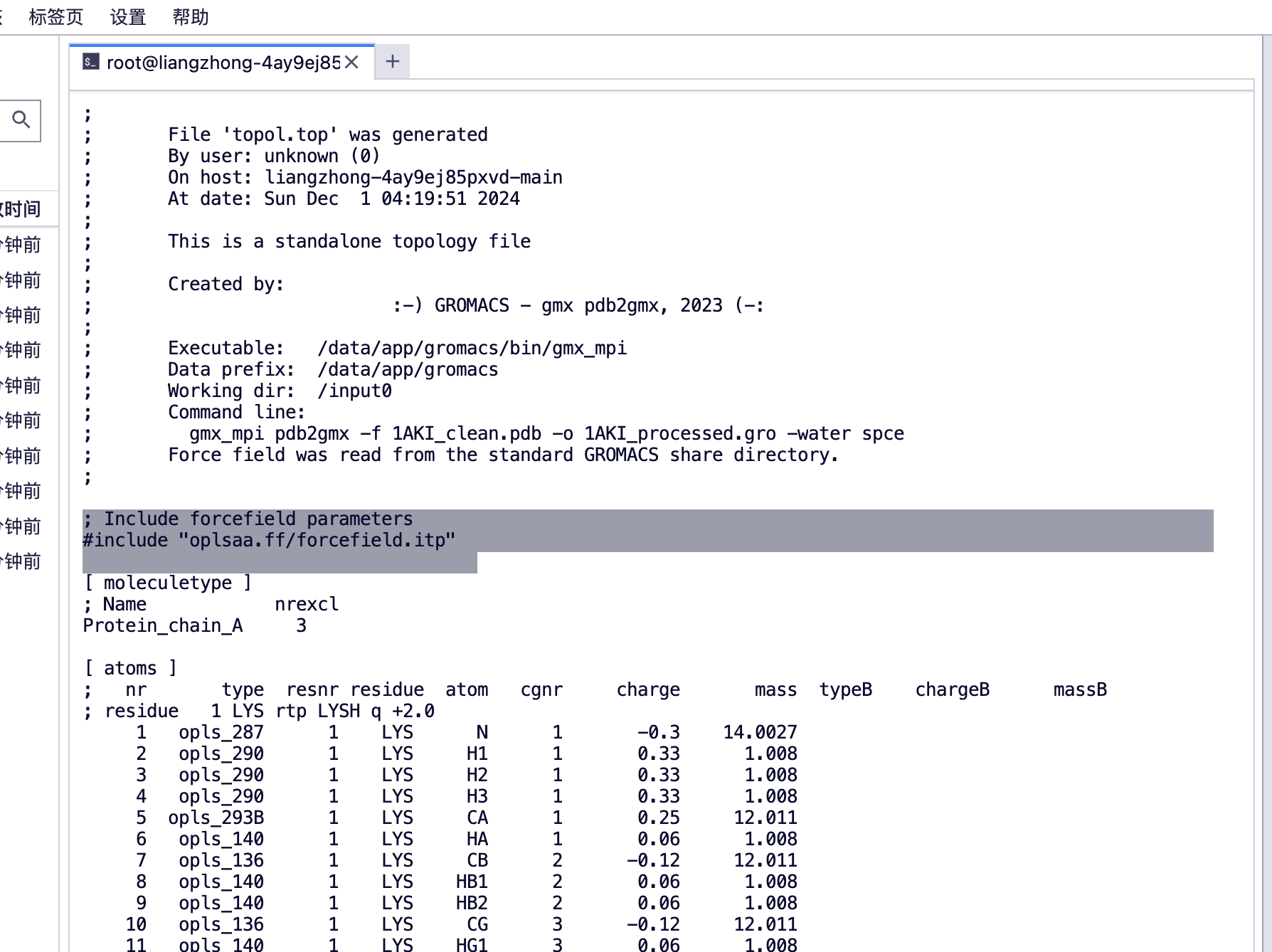
vim コマンドを使用して topol.top を表示すると、追加の力場のラベルが表示されます。
(base) root@liangzhong-4ay9ej85pxvd-main:/input0# ls
1AKI_clean.pdb      1aki.pdb  md.mdp     npt.mdp  posre.itp
1AKI_processed.gro  ions.mdp  minim.mdp  nvt.mdp  topol.top
4. 溶媒分子を追加できるように、タンパク質を覆う菱形の十二面体のボックスを作成します。
• ボックス選択: 一般的なシミュレーションボックスの形状には、立方体、直交ボックス、菱形十二面体などが含まれます。通常、分子を効果的に充填し、計算量を削減できる形状が選択されます。
gmx_mpi editconf -f 1AKI_processed.gro -o 1AKI_newbox.gro -c -d 1.0 -bt cubic

#将蛋白质在框中居中(-c),并将其放置在框边缘至少 1.0 nm 的位置(-d 1.0)

Command line:
  gmx_mpi editconf -f 1AKI_processed.gro -o 1AKI_newbox.gro -c -d 1.0 -bt cubic

Note that major changes are planned in future for editconf, to improve usability and utility.
Read 1960 atoms
Volume: 123.376 nm^3, corresponds to roughly 55500 electrons
No velocities found
    system size :  3.817  4.234  3.454 (nm)
    diameter    :  5.010               (nm)
    center      :  2.781  2.488  0.017 (nm)
    box vectors :  5.906  6.845  3.052 (nm)
    box angles  :  90.00  90.00  90.00 (degrees)
    box volume  : 123.38               (nm^3)
    shift       :  0.724  1.017  3.488 (nm)
new center      :  3.505  3.505  3.505 (nm)
new box vectors :  7.010  7.010  7.010 (nm)
new box angles  :  90.00  90.00  90.00 (degrees)
new box volume  : 344.48               (nm^3)
5. ボックスを定義し、溶媒 (水) を追加します。
目的:溶媒和: 分子を溶媒環境 (ウォーターボックスなど) に配置して、実際の環境での挙動をシミュレートします。
gmx_mpi solvate -cp 1AKI_newbox.gro -cs spc216.gro -o 1AKI_solv.gro -p topol.top

#结果
Generating solvent configuration
Will generate new solvent configuration of 4x4x4 boxes
Solvent box contains 39252 atoms in 13084 residues
Removed 5451 solvent atoms due to solvent-solvent overlap
Removed 1869 solvent atoms due to solute-solvent overlap
Sorting configuration
Found 1 molecule type:
    SOL (   3 atoms): 10644 residues
Generated solvent containing 31932 atoms in 10644 residues
Writing generated configuration to 1AKI_solv.gro

Output configuration contains 33892 atoms in 10773 residues
Volume                 :     344.484 (nm^3)
Density                :     997.935 (g/l)
Number of solvent molecules:  10644

Processing topology
Adding line for 10644 solvent molecules with resname (SOL) to topology file (topol.top)

#查看一下 top 文件
(base) root@liangzhong-4ay9ej85pxvd-main:/input0# ls
'#topol.top.1#'   1AKI_newbox.gro      1AKI_solv.gro   ions.mdp   minim.mdp   nvt.mdp     topol.top
 1AKI_clean.pdb   1AKI_processed.gro   1aki.pdb        md.mdp     npt.mdp     posre.itp
(base) root@liangzhong-4ay9ej85pxvd-main:/input0# vim topol.top
#查看 top 文件的末尾
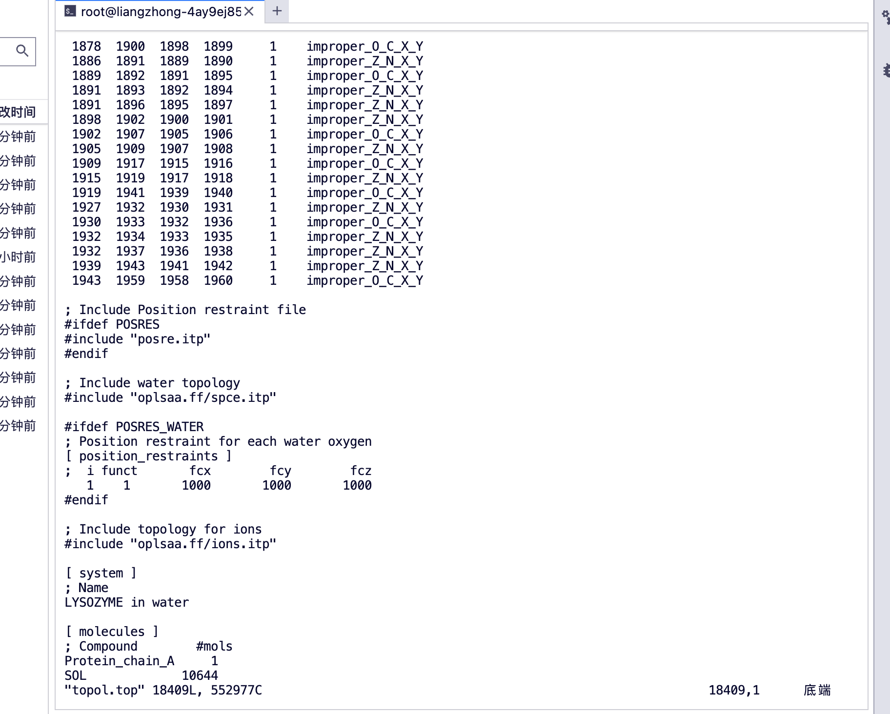
[分子]が見える
プロテイン_チェーン_A、プロテイン A チェーン
SOL水分子
6. .tpr ファイルをアセンブルします。
gmx_mpi grompp -f ions.mdp -c 1AKI_solv.gro -p topol.top -o ions.tpr
7. 電荷を中和し、溶媒分子をイオンに置き換えます。
電気的中性: イオン (Na⁺、Cl⁻ など) を追加してシステムの総電荷を中和し、静電効果によるシミュレーションの歪みを回避します。
gmx_mpi genion -s ions.tpr -o 1AKI_solv_ions.gro -p topol.top -pname NA -nname CL -neutral
Command line:
gmx_mpi genion -s ions.tpr -o 1AKI_solv_ions.gro -p topol.top -pname NA -nname CL -neutral
Reading file ions.tpr, VERSION 2023 (single precision)
Reading file ions.tpr, VERSION 2023 (single precision)
Will try to add 0 NA ions and 8 CL ions.
Select a continuous group of solvent molecules
Group 0 ( System) has 33892 elements
Group 1 ( Protein) has 1960 elements
Group 2 ( Protein-H) has 1001 elements
Group 3 ( C-alpha) has 129 elements
Group 4 ( Backbone) has 387 elements
Group 5 ( MainChain) has 517 elements
Group 6 ( MainChain+Cb) has 634 elements
Group 7 ( MainChain+H) has 646 elements
Group 8 ( SideChain) has 1314 elements
Group 9 ( SideChain-H) has 484 elements
Group 10 ( Prot-Masses) has 1960 elements
Group 11 ( non-Protein) has 31932 elements
Group 12 ( Water) has 31932 elements
Group 13 ( SOL) has 31932 elements
Group 14 ( non-Water) has 1960 elements
Select a group: 13
Selected 13: 'SOL'
Number of (3-atomic) solvent molecules: 10644
Processing topology
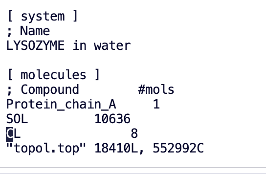
Replacing 8 solute molecules in topology file (topol.top) by 0 NA and 8 CL ions.
Back Off! I just backed up topol.top to ./#topol.top.2#
Using random seed -1212354563.
Replacing solvent molecule 3671 (atom 12973) with CL
Replacing solvent molecule 2264 (atom 8752) with CL
Replacing solvent molecule 2559 (atom 9637) with CL
Replacing solvent molecule 8081 (atom 26203) with CL
Replacing solvent molecule 8468 (atom 27364) with CL
Replacing solvent molecule 7439 (atom 24277) with CL
Replacing solvent molecule 9983 (atom 31909) with CL
Replacing solvent molecule 650 (atom 3910) with CL
GROMACS reminds you: "Water is just water" (Berk Hess)
(base) root@liangzhong-4ay9ej85pxvd-main:/input0#
塩素イオンが多く添加されているのがわかります。
8. エネルギーの最小化
8.1 理由: 分子動力学シミュレーションを実行する場合、取得する pdb ファイルは X 線や電子顕微鏡などを通じて取得されるため、過度に高エネルギーの結合角や歪みなどが多く含まれたり、水素結合の形成が含まれたりします。あるいは、破損、分子間の特別な配置、または原子間の距離が近いことによって引き起こされる高エネルギーにより、シミュレーション内の分子システムが高エネルギー状態から低エネルギー状態に遷移することが困難になります。現時点では、システムのエネルギーを最小限に抑えるためにこの方法を使用する必要があります。
8.2 原理: エネルギー最小化の基本原理: エネルギー最小化は位置エネルギー関数に基づいており、原子座標を繰り返し計算して調整することで系の総位置エネルギーを削減します。一般的に使用される方法は次のとおりです。
①共役勾配法:前ステップの情報を利用して収束を加速する勾配降下法。
②最急降下法:各反復は位置エネルギー勾配の逆方向に移動し、最急降下経路によってエネルギーを減少させます。
③ニュートン・ラフソン法:位置エネルギー関数の二階微分を用いて、エネルギー最小点をより正確に求める二次微分法。
8.3 目的: 分子の原子座標を調整することで系の総位置エネルギーを減らし、それによってより安定した分子の立体構造を見つけます。
①不合理な幾何学的配座の除去:エネルギー最小化により、不当な原子の重なりや伸縮などの初期構造の不当な幾何学的配座を除去し、それらによって引き起こされる高エネルギー状態を排除し、系をより安定化します。
② 初期構造の準備: シミュレーションプロセス中の不必要な高エネルギー衝撃を避けるために、初期構造がより低い位置エネルギー状態にあることを確認します。
③ 計算効率の向上:系の総位置エネルギーを低減することで、その後のシミュレーションや計算の安定性と効率を向上させることができます。
gmx_mpi grompp -f minim.mdp -c 1AKI_solv_ions.gro -p topol.top -o em.tpr
gmx_mpi mdrun -v -deffnm em
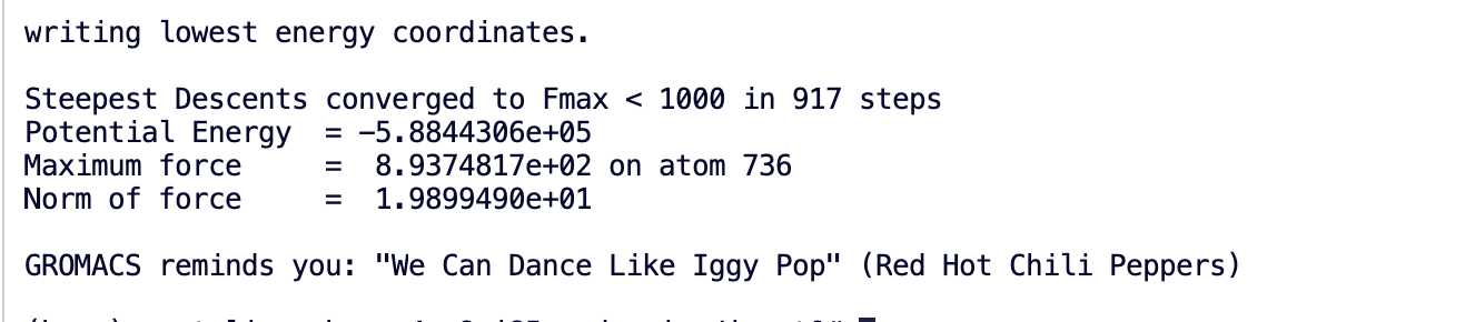
9. 結果を見てみましょう (チュートリアルの最後に、xvg ファイルを視覚化する方法を説明します。グラフを作成するには、xmgrace、qtgrace、Python、Excel を使用できます。基本的には折れ線グラフです)
gmx_mpi energy -f em.edr -o potential.xvg
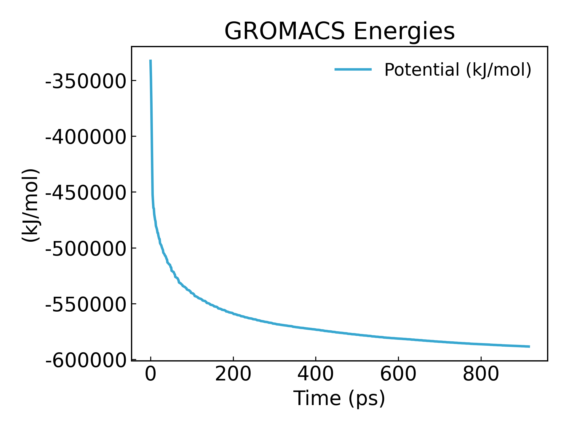
エネルギーが-600000kj/mol と最小化されていることがわかります。
10. システムバランス
目標: システムを目標の温度と圧力条件に調整して、実際の物理的状態に近づけます。
(1) NVT シミュレーション (定体積および定温度):
• 定容定温度アンサンブルは、システム温度を目標値に安定させるために使用されます。
• 温度コントローラー: 一般的には、原子速度を調整することによって温度を制御する、Berendsen 温度カプラーまたは V-rescale (修正弱結合法) が使用されます。
(2) NPT シミュレーション (一定の圧力と温度):
• 一定の圧力と温度のアンサンブルにより、システム密度が目標値 (通常は液体の水の密度 ~1 g/cm3) にさらに調整されます。
• 圧力コントローラー: 一般的には、Berendsen 圧力カプラーまたは Parrinello-Rahman 圧力制御方式が使用されます。
10.1. (一定の粒子数、体積、温度) で 100 ps の NVT 平衡化を実行します。これは「等温および等容積」とも呼ばれます。
GPU アクセラレーション下では非常に高速で、わずか 10 秒以上かかります。
gmx_mpi grompp -f nvt.mdp -c em.gro -r em.gro -p topol.top -o nvt.tpr

gmx_mpi mdrun -deffnm nvt -nb gpu -pme cpu
#将 PME 任务移至 CPU
gmx_mpi energy -f nvt.edr -o temperature.xvg
#生成温度随时间变化的图像,查看温度是否平衡
16
0
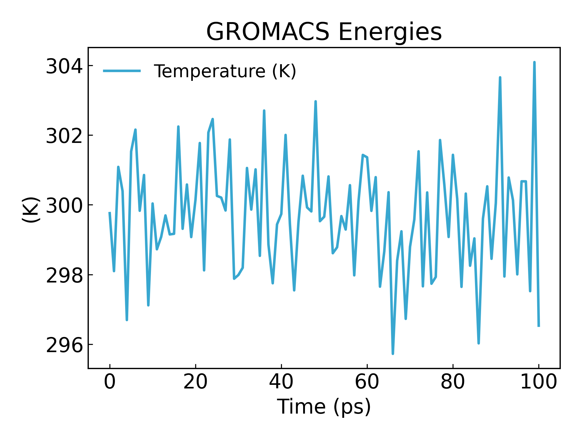
温度も 100ps 以内に基本的な定常状態に達することがわかります。
10.2.npt の「等温および等圧」平衡、システムの圧力を安定させ、100 ps の NPT 平衡を実行します。
gmx_mpi grompp -f npt.mdp -c nvt.gro -r nvt.gro -t nvt.cpt -p topol.top -o npt.tpr
gmx_mpi mdrun -deffnm npt -nb gpu -pme cpu
#压力是否平衡
gmx_mpi energy -f npt.edr -o pressure.xvg
18
0
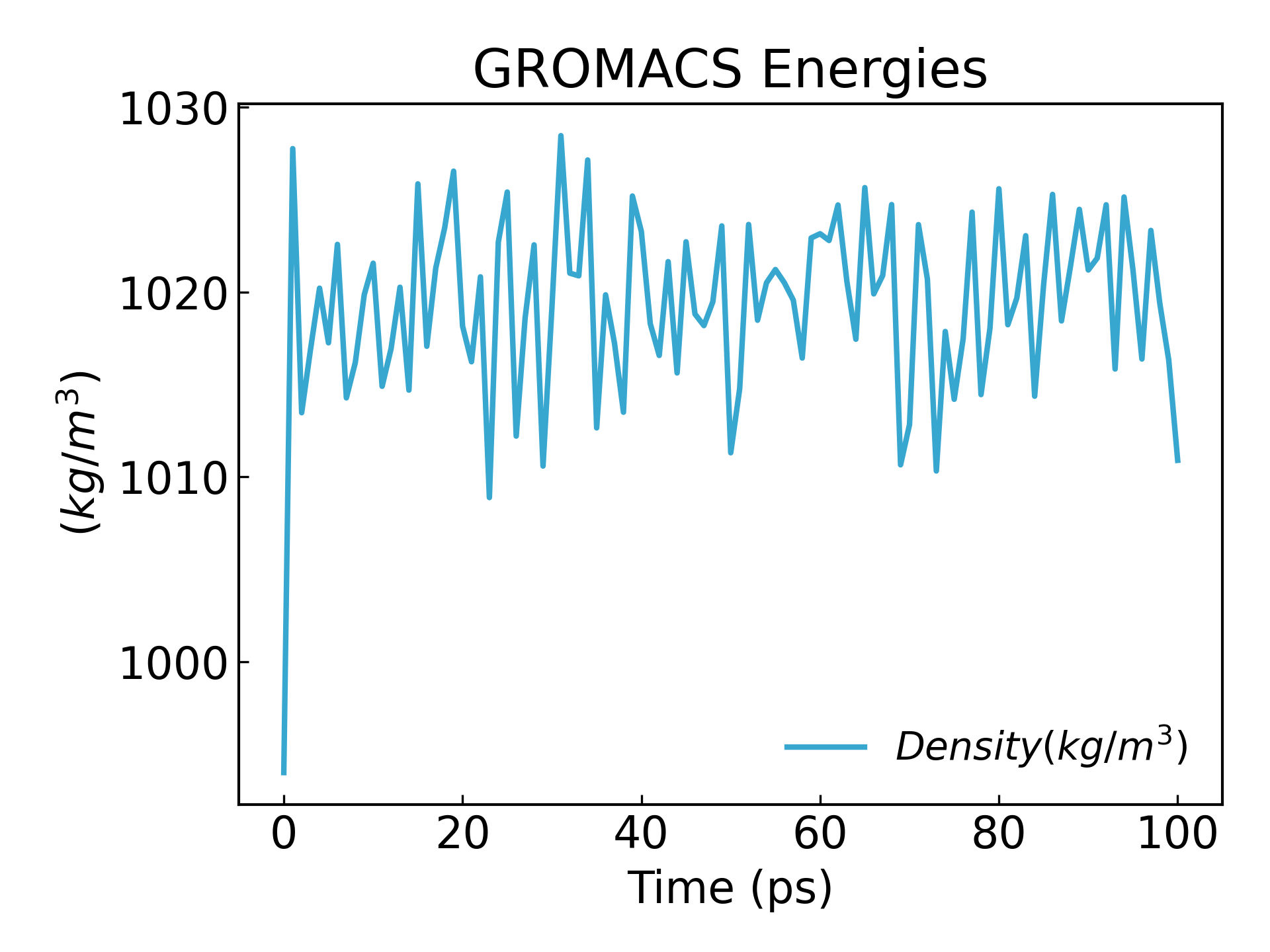
gmx_mpi energy -f npt.edr -o density.xvg
24
0
密度が定常状態に達していることがわかります。
11. 2 つの平衡段階が完了すると、システムは希望の温度と圧力で十分に平衡になります。これで、位置の制約を解除して MD を実行できるようになります。
ここで、必要に応じて時間を変更できます。このチュートリアルでは 100ns をシミュレートします。
タイムステップ dt = 2 fs (共通設定):
50000000 ステップ、時間ステップは 2 fs、100 ナノ秒 (ns) に相当
50000000 x2 fs = 10^8 fs = 10^5 ps =100ns
vim md.mdp
nsteps                  = 50000000    ; 2 * 50000000 = 100000 ps (100 ns)
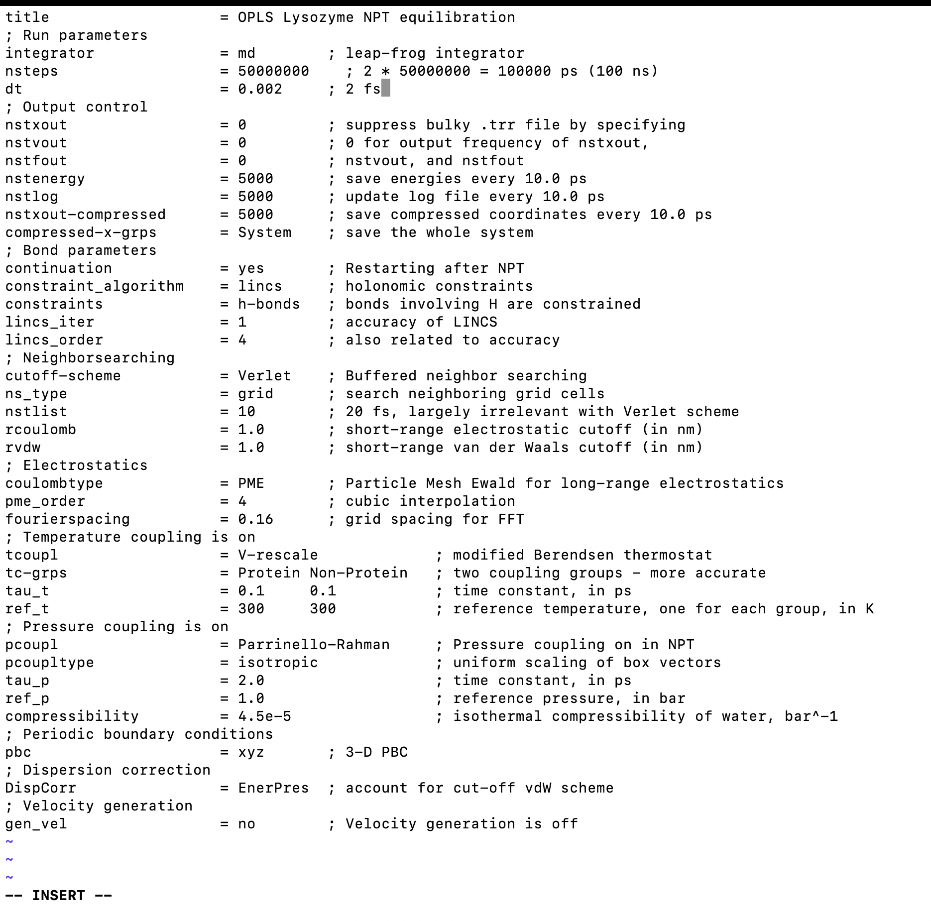
gmx_mpi grompp -f md.mdp -c npt.gro -t npt.cpt -p topol.top -o md_0_1.tpr
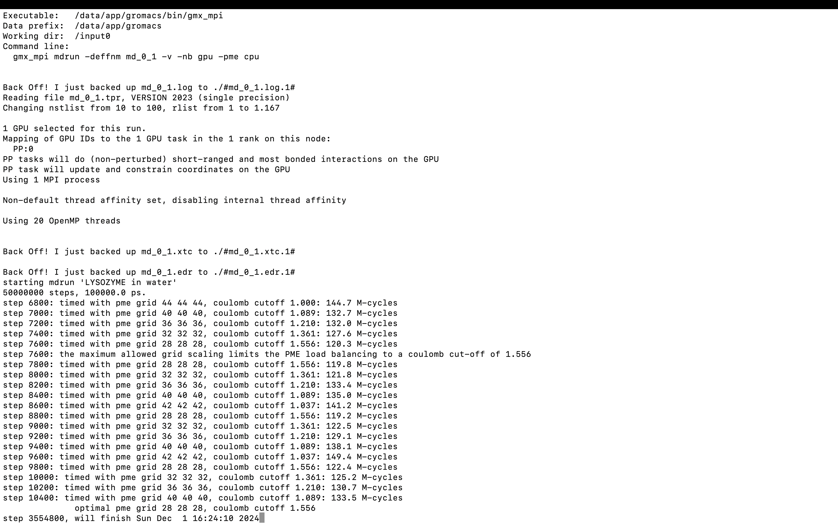
##最后一步提交,pme 分配到 CPU 上:
gmx_mpi mdrun -deffnm md_0_1 -v -nb gpu -pme cpu
-v を使用すると、実行の残り時間を表示できます。
3. 結果の分析
1.trjconv は、座標の削除、周期性の修正、または軌道 (時間単位、フレーム周波数など) の手動変更を行うための後処理ツールとして使用されます。これは、周期的な境界条件を持つすべてのシミュレーションでは、分子が壊れる可能性があるためです。または、ボックスの端の周りをジャンプして、分子をボックスの中央に再配置し、分子を再ラップして、ボックスの菱形十二面体の形状を復元することができます。
-pbc mol: 去除轨迹中的周期性边界条件 (PBC),并基于分子进行修正(即确保每个分子在轨迹中是完整的)。
•	-center: 将选定的分子/分组居中到模拟框的中心。
gmx_mpi trjconv -s md_0_1.tpr -f md_0_1.xtc -o md_0_1_noPBC.xtc -pbc mol -center

Select group for centering
Group     0 (         System) has 33876 elements
Group     1 (        Protein) has  1960 elements
Group     2 (      Protein-H) has  1001 elements
Group     3 (        C-alpha) has   129 elements
Group     4 (       Backbone) has   387 elements
Group     5 (      MainChain) has   517 elements
Group     6 (   MainChain+Cb) has   634 elements
Group     7 (    MainChain+H) has   646 elements
Group     8 (      SideChain) has  1314 elements
Group     9 (    SideChain-H) has   484 elements
Group    10 (    Prot-Masses) has  1960 elements
Group    11 (    non-Protein) has 31916 elements
Group    12 (          Water) has 31908 elements
Group    13 (            SOL) has 31908 elements
Group    14 (      non-Water) has  1968 elements
Group    15 (            Ion) has     8 elements
Group    16 ( Water_and_ions) has 31916 elements
Select a group: 1
Selected 1: 'Protein'
Select group for output
Group     0 (         System) has 33876 elements
Group     1 (        Protein) has  1960 elements
Group     2 (      Protein-H) has  1001 elements
Group     3 (        C-alpha) has   129 elements
Group     4 (       Backbone) has   387 elements
Group     5 (      MainChain) has   517 elements
Group     6 (   MainChain+Cb) has   634 elements
Group     7 (    MainChain+H) has   646 elements
Group     8 (      SideChain) has  1314 elements
Group     9 (    SideChain-H) has   484 elements
Group    10 (    Prot-Masses) has  1960 elements
Group    11 (    non-Protein) has 31916 elements
Group    12 (          Water) has 31908 elements
Group    13 (            SOL) has 31908 elements
Group    14 (      non-Water) has  1968 elements
Group    15 (            Ion) has     8 elements
Group    16 ( Water_and_ions) has 31916 elements
Select a group: 0
Selected 0: 'System'
最小二乗フィッティングと RMSD 計算には 4 (「スケルトン」) を選択します。
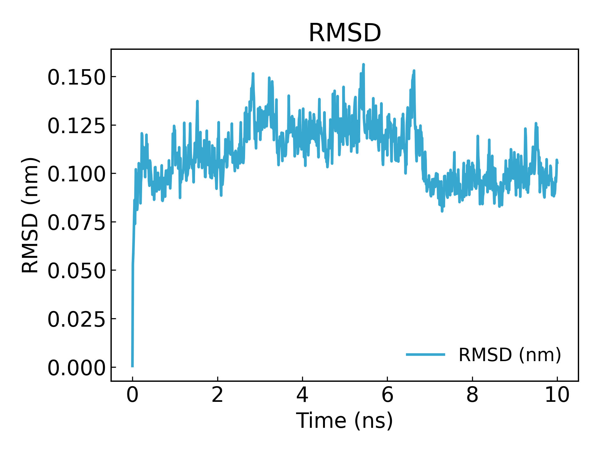
2.RMSD
** を使用して、シミュレーションの収束とタンパク質の安定性を確認するために使用できます。g_rms**シミュレーションプロセス中の構造と初期構造のRMSDを計算します。タンパク質の構造の安定性を評価するためによく使用されます。タンパク質のリガンド構造の安定性など、RMSD曲線の変動幅は小さく安定しており、リガンドと受容体との親和性が高いことを示しています。
gmx_mpi rms -s md_0_1.tpr -f md_0_1_noPBC.xtc -o rmsd.xvg
最小二乗フィッティングと RMSD 計算には 4 (「スケルトン」) を選択します。
10ns 後に平衡に達していることがわかります (注: 記事を公開または送信する場合は、時間を 100ns または 50ns までシミュレートするのが最善です)。
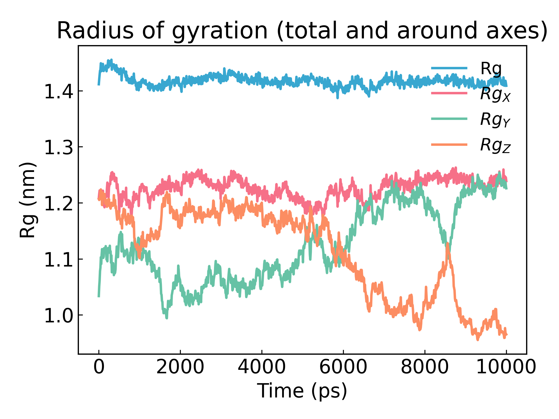
3. 回転半径の解析
gmx_mpi gyrate -s md_0_1.tpr -f md_0_1_noPBC.xtc -o gyrate.xvg
タンパク質の回転半径は、そのコンパクトさの尺度です。タンパク質の構造が安定している場合、比較的安定した Rg 値が維持される可能性があります。タンパク質が展開すると、その R g 値は時間の経過とともに変化します。シミュレーションでリゾチームの回転半径を分析してみましょう。
4. ビジュアルマッピング
推奨ソフトウェア:DuIvyTools: GROMACS シミュレーション分析および視覚化ツール
から:https://github.com/CharlesHahn/DuIvyTools
pip install DuIvyTools

dit xvg_show -f rmsd.xvg -o rmsd_plot.png

dit xvg_show -f rmsd.xvg -o rmsd_plot.png

dit xvg_show -f potential.xvg -o potential_plot.png

dit xvg_show -f temperature.xvg -o temperature_plot.png

dit xvg_show -f density.xvg -o density_plot.png
dit xvg_show -f pressure.xvg -o pressure_plot.png
自分で作成したデータセットを開く
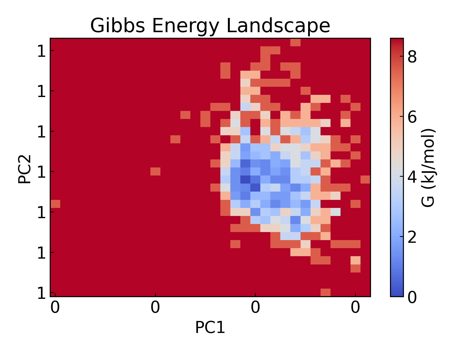
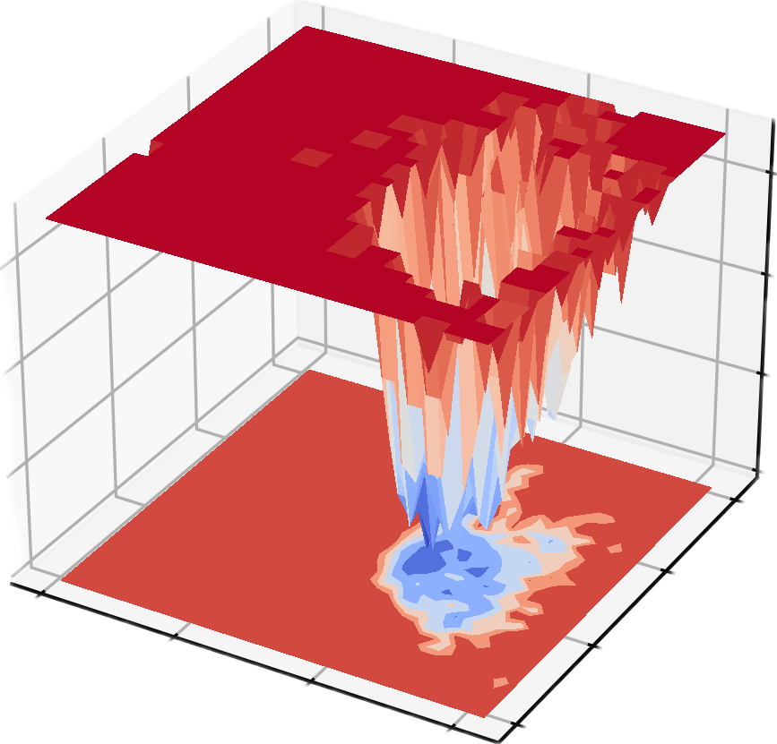
5. GROMACS は、回転半径と rmsd をそれぞれ 2 つの PCA コンポーネントとして使用して、エネルギーランドスケープ図と自由エネルギートポグラフィー図を描画します。
gmx_mpi gyrate -s md_0_1.tpr -f md_0_1_noPBC.xtc -o rg.xvg
gmx_mpi rms -s md_0_1.tpr -f md_0_1_noPBC.xtc -o rmsd.xvg
vim rmsd.xvg
#输入以下命令删除以 # 或 @ 开头的行:
:g/^[@#]/d

vim rg.xvg
#输入以下命令删除以 # 或 @ 开头的行:
:g/^[@#]/d

#注意不要有空行,
paste rmsd.xvg rg.xvg > rmsd-rg.xvg

(base) # tail -f rmsd-rg.xvg
9910.0000000    0.0925907	      9910     1.37624     1.20925     1.20765    0.931324
9920.0000000    0.0881348	      9920     1.38369     1.22248     1.21078    0.932077
9930.0000000    0.0911074	      9930     1.39224     1.23799     1.21709    0.928842
9940.0000000    0.0893596	      9940     1.38188     1.21942     1.21672    0.922916
9950.0000000    0.0915931	      9950     1.37509     1.21939     1.20194    0.922051
9960.0000000    0.0978161	      9960     1.38113      1.2262     1.21084    0.919414
9970.0000000    0.0954911	      9970     1.37934     1.21241     1.20711    0.937075
9980.0000000    0.0993617	      9980     1.38301     1.22353     1.21083     0.92862
9990.0000000    0.1069279	      9990     1.37943     1.22317     1.20579    0.924978
10000.0000000    0.1055321	     10000     1.37524     1.21648     1.20194     0.92632
^Z
[11]+  Stopped                 tail -f rmsd-rg.xvg
#查看已经将两个文件整合在一起了,我们只要保留
#从 rmsd-rg.xvg 文件内容可以看到,每一行的数据格式如下:
时间_RMSD(ns)    RMSD	      时间_Rg(ps)     Rg 其他列

(base) tail -f rmsd.xvg
9910.0000000    0.0925907
9920.0000000    0.0881348
9930.0000000    0.0911074
9940.0000000    0.0893596
9950.0000000    0.0915931
9960.0000000    0.0978161
9970.0000000    0.0954911
9980.0000000    0.0993617
9990.0000000    0.1069279
10000.0000000    0.1055321
^Z
[12]+  Stopped                 tail -f rmsd.xvg

#整理数据为
时间 (ns)    RMSD    Rg

(base) python
Python 3.8.15 (default, Nov 24 2022, 15:19:38)
[GCC 11.2.0] :: Anaconda, Inc. on linux
Type "help", "copyright", "credits" or "license" for more information.
# 加载数据
>>> import pandas as pd
>>> data = pd.read_csv("rmsd-rg.xvg", delim_whitespace=True, header=None, comment="#")
# 保留需要的列:第 1 列 (RMSD 时间) 、第 2 列 (RMSD) 、第 4 列 (Rg)
>>> cleaned_data = data[[0, 1, 3]]
# 将列名修改为更直观的名称
>>> cleaned_data.columns = ["Time (ps)", "RMSD", "Rg"]
>>> cleaned_data.to_csv("rmsd-rg-cleaned.xvg", sep="\t", index=False, header=False)
>>> exit()

#整理成功
tail -f rmsd-rg-cleaned.xvg
9910.0	0.0925907	1.37624
9920.0	0.0881348	1.38369
9930.0	0.0911074	1.39224
9940.0	0.0893596	1.38188
9950.0	0.0915931	1.37509
9960.0	0.0978161	1.38113
9970.0	0.0954911	1.37934
9980.0	0.0993617	1.38301
9990.0	0.1069279	1.37943
10000.0	0.1055321	1.37524

gmx_mpi sham -tsham 300 -nlevels 100 -f rmsd-rg-cleaned.xvg -ls gibbs.xpm -g gibbs.log -lsh enthalpy.xpm -lss entropy.xpm

dit xpm_show -f gibbs.xpm  -o gibbs_2d.png
dit xpm_show -f gibbs.xpm -m 3d -o gibbs_3d.png
#tsham : 设定温度
#-nlevels: 设定 FEL 的层次数量
フリー エネルギー ランドスケープ (FES) は、分子シミュレーションにおいて非常に重要なツールであり、主に特定の座標における分子システムの自由エネルギー分布を記述するために使用されます。その中心的な機能は、システムの熱力学的安定性と運動プロセスを明らかにすることであり、これは通常、以下の科学研究分野において非常に重要です。
- 定常状態と遷移状態の研究: システムの安定な構造 (自由エネルギーの最低点) と構造変換経路 (自由エネルギー障壁) を明らかにします。これは、タンパク質のフォールディング、化学反応、分子認識プロセスの分析に使用できます。
- 運動経路と熱力学的安定性: 異なる状態間の自由エネルギーの差を定量化し、分子の相互作用や構造遷移のエネルギー駆動を理解するのに役立ちます。
- 薬剤設計と触媒研究: リガンドと受容体の結合経路、エネルギー障壁、反応速度を予測し、分子機構の解析と機能の最適化に理論的な指針を提供します。
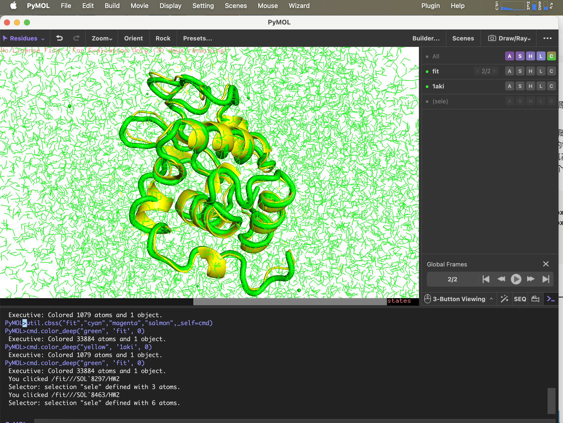
6.g_confrms 構造の違いを比較する
シミュレーション完了後の構造を最初の PDB ファイルの構造と比較するには、fit.pdb 2 つの分子構造を含むファイル (両方とも選択) 4 (Backbone)
gmx_mpi confrms -f1 1AKI_clean.pdb -f2 md_0_1.gro -o fit.pdb
pymolでpdb構造を開く
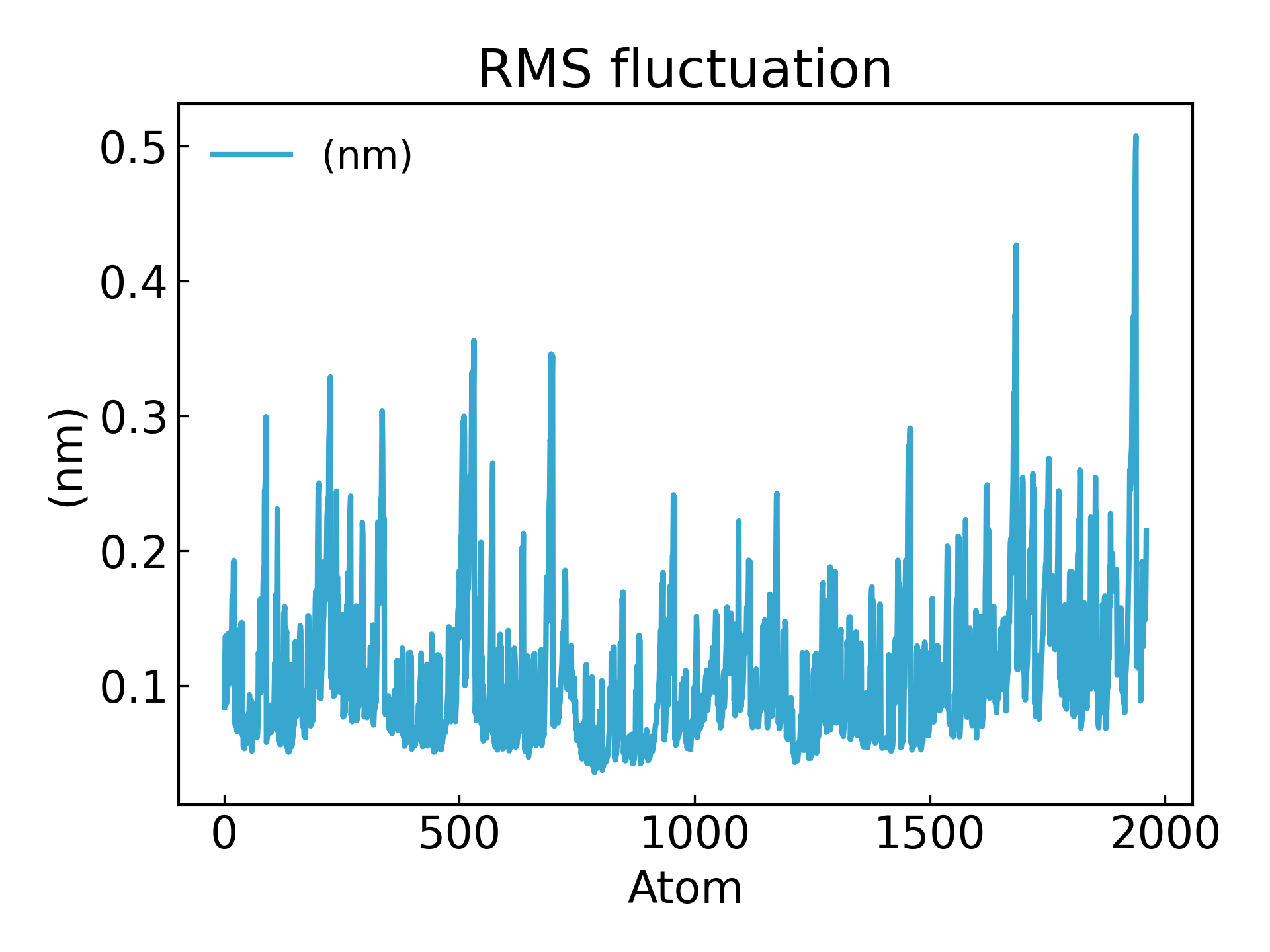
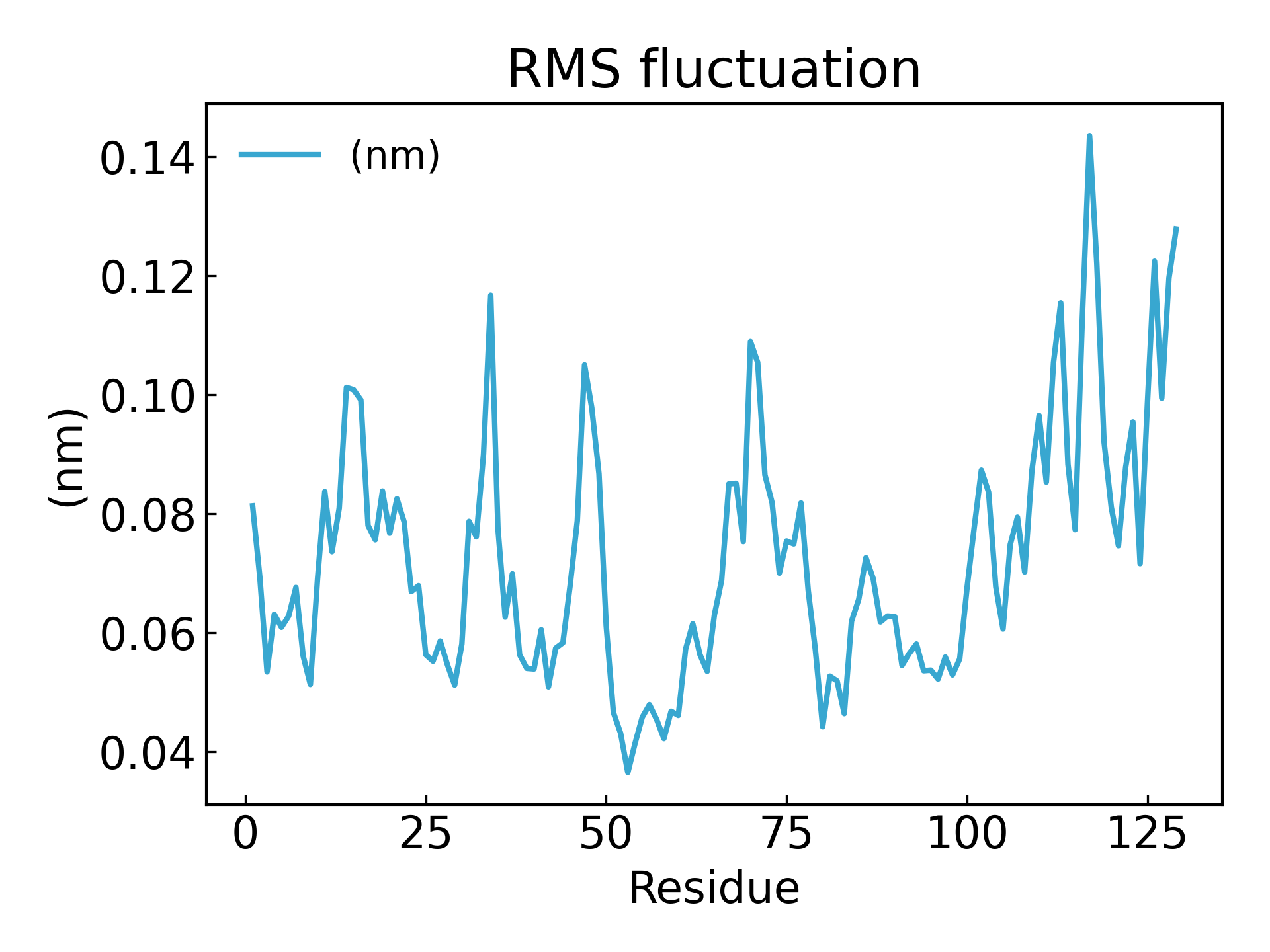
7.g_rmsf 二乗平均平方根変動RMSFを計算し、500 psの範囲内の平均構造を計算します。g_rmsf 得られるのは原子番号に応じて変化する曲線です。 1 Protein
アミノ酸残基の変動は、時間の経過に伴う各アミノ酸残基/各原子の基準位置からの平均偏差を考慮した RMSF パラメーターによって推測できます。むしろ、平均的な構造から変動するタンパク質の構造の特定の部分を分析すると言えます。 RMSF値が高いアミノ酸またはアミノ酸グループは複合体の柔軟性が高いことを示し、RMSF値が低いアミノ酸は複合体の柔軟性が低いことを示します。頻繁な変動は安定性を悪化させます。RMSF 値は、各残基位置の平均骨格柔軟性を測定する動的パラメータです [19]。
gmx_mpi rmsf -s md_0_1.tpr -f md_0_1_noPBC.xtc -b 500 -o fws-rmsf.xvg -ox fws-avg.pdb
gmx_mpi rmsf -s md_0_1.tpr -f md_0_1_noPBC.xtc -b 500 -o fws-rmsf.xvg -ox fws-avg.pdb -res

dit xvg_show -f fws-rmsf.xvg -o rmsf_res.png
# 最后可以放到 pymol 里面看轨迹动画,点击播放即可
gmx_mpi trjconv -s md_0_1.tpr -f md_0_1_noPBC.xtc -o trajectory.pdb -skip 10