Command Palette
Search for a command to run...
VASP Hybrid Functional Calculation of Silicon Density of States and Energy Bands
Vienna Ab initio Simulation Package (VASP) It is a computer program for atomic-scale material modeling from first principles, such as electronic structure calculations and quantum mechanical molecular dynamics.
VASP is suitable for calculating approximate solutions to the many-body Schrödinger equation. It covers a variety of computational methods, including solving the Kohn-Sham equation within the framework of density functional theory (DFT) and treating the Roothaan equation in the Hartree-Fock (HF) approximation. Another innovation of VASP is that it integrates the Hartree-Fock method with density functional theory to form a hybrid functional method, which provides researchers with more flexible computational options. In addition, VASP also provides Green's function methods (GW quasiparticles and ACFDT-RPA) and many-body perturbation theory (second-order Møller-Plesset).
In VASP, central quantities such as single electron orbitals, electron charge density, and local potentials are represented in plane wave basis sets. The interactions between electrons and ions are described using norm conservation or ultrasoft pseudopotentials or projector augmented wave methods.
To determine the electronic ground state, VASP makes use of efficient iterative matrix diagonalization techniques such as the residual minimization method with direct inversion iterated subspace (RMM-DIIS) or the block Davidson algorithm. These are combined with the efficient Broyden and Pulay density mixing scheme to speed up the self-consistent loop.
Tutorial Introduction
This tutorial will learn how to calculate silicon energy bands using hybrid functionals, which is similar to the previous tutorial (VASP Getting Started Tutorial: Calculating Density of States and Bandwidths in Silicon), the hybrid functional can calculate the energy bands and state density of the material with the correct band gap, but it requires more computing resources, so the GPU is used for demonstration this time.
By following this tutorial, you will learn to generate INCAR and KPOITNS required for VASP hybrid functional calculations.
Previous tutorial (VASP Getting Started Tutorial: Calculating Density of States and Bandwidths in Silicon) contains 4 steps. However, the calculation of this hybrid functional only requires 1 step (structural optimization will be skipped) to obtain the state density and energy band of silicon.
Preparing input files
This tutorial requires the preparation of four files: INCAR, POSCAR, KPOINTS and POTCAR.
INCAR
Global Parameters
  ENCUT  =  300          (波函数截断能量)
  PREC   =  Normal       (精度设置)
  LWAVE  = .TRUE.        (保存波函数)
  LCHARG = .TRUE.        (保存电荷)
  ADDGRID= .TRUE.        (增加格点加速收敛)


Static Calculation
  ISMEAR =  0            (高斯占据数)
  SIGMA  =  0.1          (高斯展宽)
  LORBIT =  11           (输出 DOSCAR 和 PROCAR)
  NELM   =  60           (最大电子步)
  EDIFF  =  1E-08        (电子步收敛判据)

HSE06 Calculation
  LHFCALC= T            (启动杂化泛函计算)
  AEXX   =  0.25        (杂化比例 0.25)
  HFSCREEN= 0.2         (杂化屏蔽参数 0.2)
  ALGO   =  ALL         (最优化算法)
  TIME   =  0.4         (最优化算法步长)
  PRECFOCK= N           (FFT 精度)
POSCAR
Si #(体系名称)
1.0 #(放大系数  下面 3 行对应 3 个晶格矢量 )
0.0 2.75 2.75
2.75 0.0 2.75
2.75 2.75 0.0
Si #(元素)
2 #(对应元素原子数)
Direct #(采用分数坐标,下列为 2 个原子的分数坐标)
0 0 0
0.25 0.25 0.25
KPOINTS
0.060   5   5   5   10  0.060   83    6   19    6   20   16   13    9           # Parameters to Generate KPOINTS (Do NOT Edit This Line)
    93
Reciprocal lattice
    0.00000000000000    0.00000000000000    0.00000000000000     1
    0.20000000000000    0.00000000000000    0.00000000000000     8
    0.40000000000000    0.00000000000000    0.00000000000000     8
    0.20000000000000    0.20000000000000    0.00000000000000     6
    0.40000000000000    0.20000000000000    0.00000000000000    24
   -0.40000000000000    0.20000000000000    0.00000000000000    24
   -0.20000000000000    0.20000000000000    0.00000000000000    12
    0.40000000000000    0.40000000000000    0.00000000000000     6
   -0.40000000000000    0.40000000000000    0.00000000000000    12
   -0.40000000000000    0.40000000000000    0.20000000000000    24 (以上为 scf 点位)
    0.00000000000000    0.00000000000000    0.00000000000000     0 (以下为能带点位)
    0.02777777777778    0.00000000000000    0.02777777777778     0
    0.05555555555556    0.00000000000000    0.05555555555556     0
    0.08333333333333    0.00000000000000    0.08333333333333     0
    0.11111111111111    0.00000000000000    0.11111111111111     0
    0.13888888888889    0.00000000000000    0.13888888888889     0
    0.16666666666667    0.00000000000000    0.16666666666667     0
    0.19444444444444    0.00000000000000    0.19444444444444     0
    0.22222222222222    0.00000000000000    0.22222222222222     0
    0.25000000000000    0.00000000000000    0.25000000000000     0
    0.27777777777778    0.00000000000000    0.27777777777778     0
    0.30555555555556    0.00000000000000    0.30555555555556     0
    0.33333333333333    0.00000000000000    0.33333333333333     0
    0.36111111111111    0.00000000000000    0.36111111111111     0
    0.38888888888889    0.00000000000000    0.38888888888889     0
    0.41666666666667    0.00000000000000    0.41666666666667     0
    0.44444444444444    0.00000000000000    0.44444444444444     0
    0.47222222222222    0.00000000000000    0.47222222222222     0
    0.50000000000000    0.00000000000000    0.50000000000000     0
    0.50000000000000    0.00000000000000    0.50000000000000     0
    0.52500000000000    0.05000000000000    0.52500000000000     0
    0.55000000000000    0.10000000000000    0.55000000000000     0
    0.57500000000000    0.15000000000000    0.57500000000000     0
    0.60000000000000    0.20000000000000    0.60000000000000     0
    0.62500000000000    0.25000000000000    0.62500000000000     0
    0.37500000000000    0.37500000000000    0.75000000000000     0
    0.35526315789474    0.35526315789474    0.71052631578947     0
    0.33552631578947    0.33552631578947    0.67105263157895     0
    0.31578947368421    0.31578947368421    0.63157894736842     0
    0.29605263157895    0.29605263157895    0.59210526315789     0
    0.27631578947368    0.27631578947368    0.55263157894737     0
    0.25657894736842    0.25657894736842    0.51315789473684     0
    0.23684210526316    0.23684210526316    0.47368421052632     0
    0.21710526315789    0.21710526315789    0.43421052631579     0
    0.19736842105263    0.19736842105263    0.39473684210526     0
    0.17763157894737    0.17763157894737    0.35526315789474     0
    0.15789473684211    0.15789473684211    0.31578947368421     0
    0.13815789473684    0.13815789473684    0.27631578947368     0
    0.11842105263158    0.11842105263158    0.23684210526316     0
    0.09868421052632    0.09868421052632    0.19736842105263     0
    0.07894736842105    0.07894736842105    0.15789473684211     0
    0.05921052631579    0.05921052631579    0.11842105263158     0
    0.03947368421053    0.03947368421053    0.07894736842105     0
    0.01973684210526    0.01973684210526    0.03947368421053     0
    0.00000000000000    0.00000000000000    0.00000000000000     0
    0.00000000000000    0.00000000000000    0.00000000000000     0
    0.03333333333333    0.03333333333333    0.03333333333333     0
    0.06666666666667    0.06666666666667    0.06666666666667     0
    0.10000000000000    0.10000000000000    0.10000000000000     0
    0.13333333333333    0.13333333333333    0.13333333333333     0
    0.16666666666667    0.16666666666667    0.16666666666667     0
    0.20000000000000    0.20000000000000    0.20000000000000     0
    0.23333333333333    0.23333333333333    0.23333333333333     0
    0.26666666666667    0.26666666666667    0.26666666666667     0
    0.30000000000000    0.30000000000000    0.30000000000000     0
    0.33333333333333    0.33333333333333    0.33333333333333     0
    0.36666666666667    0.36666666666667    0.36666666666667     0
    0.40000000000000    0.40000000000000    0.40000000000000     0
    0.43333333333333    0.43333333333333    0.43333333333333     0
    0.46666666666667    0.46666666666667    0.46666666666667     0
    0.50000000000000    0.50000000000000    0.50000000000000     0
    0.50000000000000    0.50000000000000    0.50000000000000     0
    0.50000000000000    0.47916666666667    0.52083333333333     0
    0.50000000000000    0.45833333333333    0.54166666666667     0
    0.50000000000000    0.43750000000000    0.56250000000000     0
    0.50000000000000    0.41666666666667    0.58333333333333     0
    0.50000000000000    0.39583333333333    0.60416666666667     0
    0.50000000000000    0.37500000000000    0.62500000000000     0
    0.50000000000000    0.35416666666667    0.64583333333333     0
    0.50000000000000    0.33333333333333    0.66666666666667     0
    0.50000000000000    0.31250000000000    0.68750000000000     0
    0.50000000000000    0.29166666666667    0.70833333333333     0
    0.50000000000000    0.27083333333333    0.72916666666667     0
    0.50000000000000    0.25000000000000    0.75000000000000     0
    0.50000000000000    0.25000000000000    0.75000000000000     0
    0.50000000000000    0.21875000000000    0.71875000000000     0
    0.50000000000000    0.18750000000000    0.68750000000000     0
    0.50000000000000    0.15625000000000    0.65625000000000     0
    0.50000000000000    0.12500000000000    0.62500000000000     0
    0.50000000000000    0.09375000000000    0.59375000000000     0
    0.50000000000000    0.06250000000000    0.56250000000000     0
    0.50000000000000    0.03125000000000    0.53125000000000     0
    0.50000000000000    0.00000000000000    0.50000000000000     0
POTCAR
The system corresponds to the pseudopotential combination of elements, here it is the pseudopotential of Si.
Run steps
Next, we will move on to the practical part of the tutorial. The tutorial has prepared the required packages, and you can directly clone the container. This tutorial uses RTX 4090 computing resources, vasp 6.3.0-cuda11.8 version image, and operates in the workspace.
1. Clone and start the container
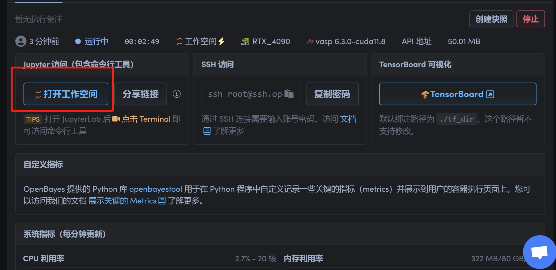
1.1 Wait for the container to load and then click Open Workspace
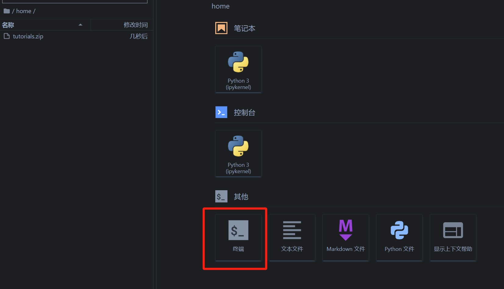
1.2 Open Terminal
1.3 Enter the wfl directory
cd tutorials/wfl
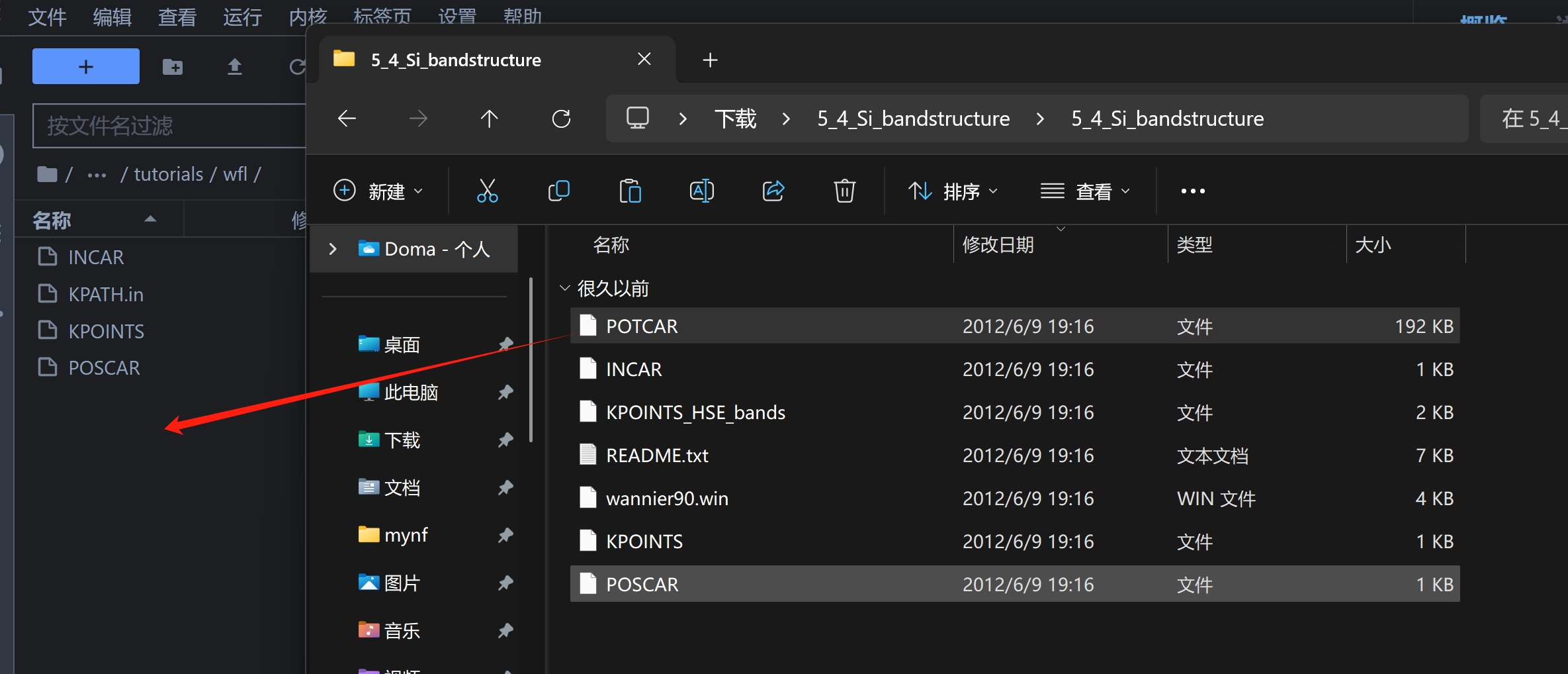
1.4 Upload the prepared silicon pseudopotential to the wfl directory
Here you can useOfficial website sample filePseudopotential POTCAR
2. Run VASP
mpirun -n 1 vasp_std
3. Install vaspkit
Return to the previous directory
cd ..
3.1 Install Python dependencies
pip install numpy scipy matplotlib
3.2 Configure vaspkit
chmod 777 setupvk.sh
./setupvk.sh
source ~/.bashrc
cd tutorials
4. Processing data using vaspkit
4.1 Plotting the Density of States and Band Diagrams
Enter the wfl directory by typing:
cd wfl
Enter the command to generate state density data:
vaspkit
111
1
Enter the command to use vaspkit to process the band data and plot it:
vaspkit
252
2
The density of states and band diagram can be generated:
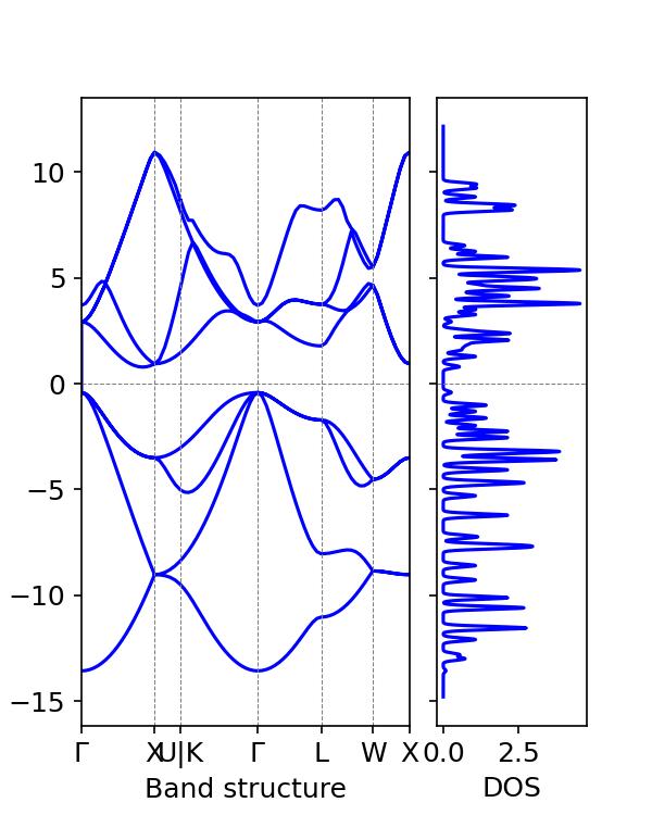
Let's use vaspkit to view the band gap:
vaspkit
911
It can be obtained that the estimated silicon band gap is 1.2eV, which is close to the typical silicon band gap experimental value of 1.12eV.
In the previous tutorial, DFT calculations using vaspkit revealed a band gap of 0.6133 eV, which is far from the experimental value.
Therefore, hybrid functionals can calculate the band gap of materials more accurately, but they require more computing resources.
Build AI with AI
From idea to launch — accelerate your AI development with free AI co-coding, out-of-the-box environment and best price of GPUs.