Command Palette
Search for a command to run...
LAMMPS Getting Started Tutorial: Estimating the Melting Point of FCC Cu Using Npt Temperature Control
LAMMPS, short for Large-scale Atomic/Molecular Massively Parallel Simulator, is a classic molecular dynamics simulation code that focuses on material modeling. It is designed to run efficiently on parallel computers and to be easily extended and modified. LAMMPS was originally developed by Sandia National Laboratories, an agency of the U.S. Department of Energy, and now includes contributions from many research groups and individuals from many institutions.
本教程使用 LAMMPS CPU 即可运行。

通过本教程的学习,您将能够:

* 理解 npt 控温操作流程
* 使用 dump 和 fix 指令将数据预处理
Effect examples

1. Preparation before operation
Here we first introduce some input files, potential function types and npt temperature control processes that need to be used.
1. Input File
Enter ./melt_u3, the melt.in file is as follows:
units            real
dimension        3
boundary         p p p


atom_style    atomic
# 读取铜结构
read_data      cu


#选用 eam potential
pair_style       eam
pair_coeff      * *  Cu_u3.eam

#每隔 100 时间步长于屏幕输出
thermo            100
thermo_style      custom step temp pe press vol lx density
#将原子轨迹输出到文件 md.lammpstrj
dump              2 all custom 100 md.lammpstrj id type x y z


#结构优化
minimize       1.0e-10 1.0e-10 10000 10000

#nvt 压强弛豫
fix                  1      all   nvt temp 1000 1000 100
run                 10000
unfix                1

#npt 体积弛豫
fix                  1      all npt temp 1000 1000 100 iso 1 1 1000
run                 10000
unfix              1


#将温度和体积量分别存储到 t 和 v 中
variable t equal "temp"
variable v equal "vol"


#npt 控温由 1000K 升温至 2000K 。
#升温速率为 (2000-1000)/100000=0.001 K/fs=1K/ps
fix                  1 all npt temp 1000 2000 100 iso 1 1 1000
fix                  2 all ave/time 100 10 10000 v_t v_v file t_v.txt
run                1000000
2. Potential function type
This project provides a demonstration model of the eam potential function
eam
./melt_u3
Corresponding potential function module
pair_style       eam
pair_coeff      * *  Cu_u3.eam
3.npt temperature control process
The main process is:
nvt pressure relaxation, npt volume relaxation
#结构优化
minimize       1.0e-10 1.0e-10 10000 10000

#nvt 压强弛豫
fix                  1      all   nvt temp 1000 1000 100
run                 10000
unfix                1

#npt 体积弛豫
fix                  1      all npt temp 1000 1000 100 iso 1 1 1000
run                 10000
unfix              1
npt heating
#npt 控温由 1000K 升温至 2000K 。
#升温速率为 (2000-1000)/100000=0.001 K/fs=1K/ps
fix                  1 all npt temp 1000 2000 100 iso 1 1 1000
fix                  2 all ave/time 100 10 10000 v_t v_v file t_v.txt
run                1000000
2. Practical operation steps (taking CPU as an example)
1. Create and start a container molecular dynamics simulation
1.1 Open the OpenBayes personal user interface, click "High Performance Computing" on the left > "Create New Container" in the upper right corner
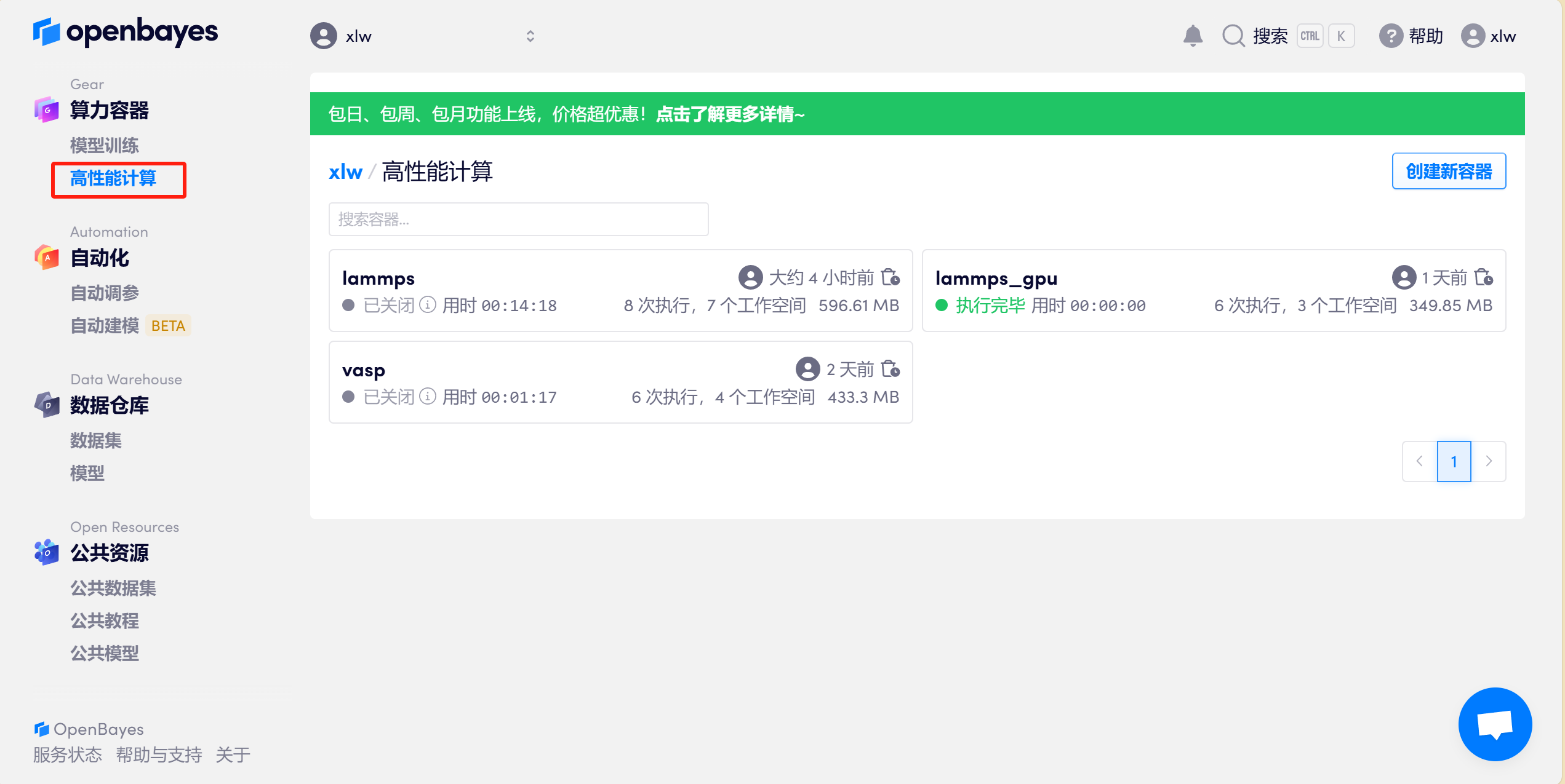
1.2 Computing power Select "CPU" > "lammps-2024-cpu" and give a container name, such as lammps > Select "Workspace" and click "Next: Select computing power"
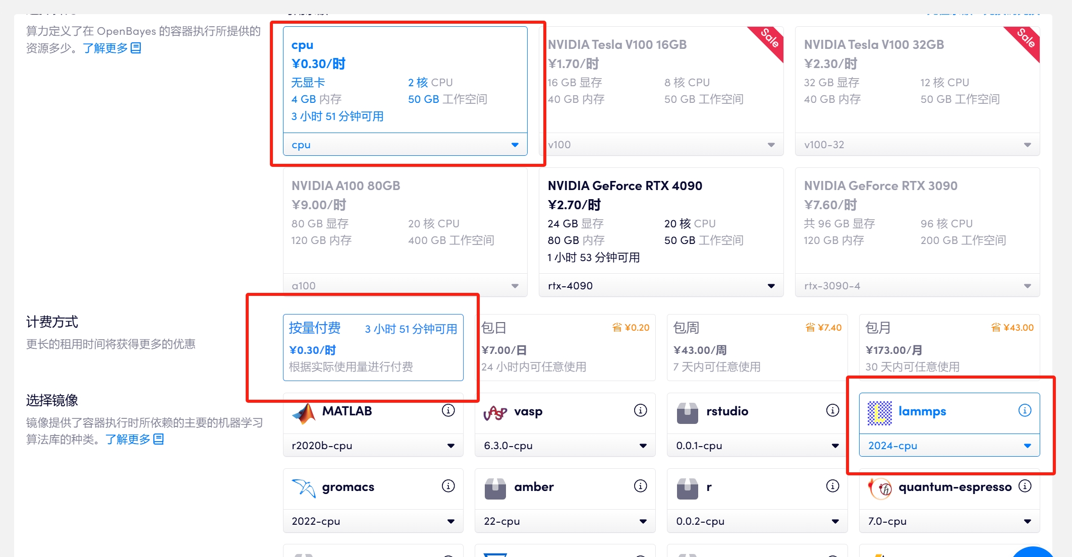
1.3 Give a container name, such as lammps > Select "Workspace" and click "Execute"

2. Conduct molecular dynamics simulation
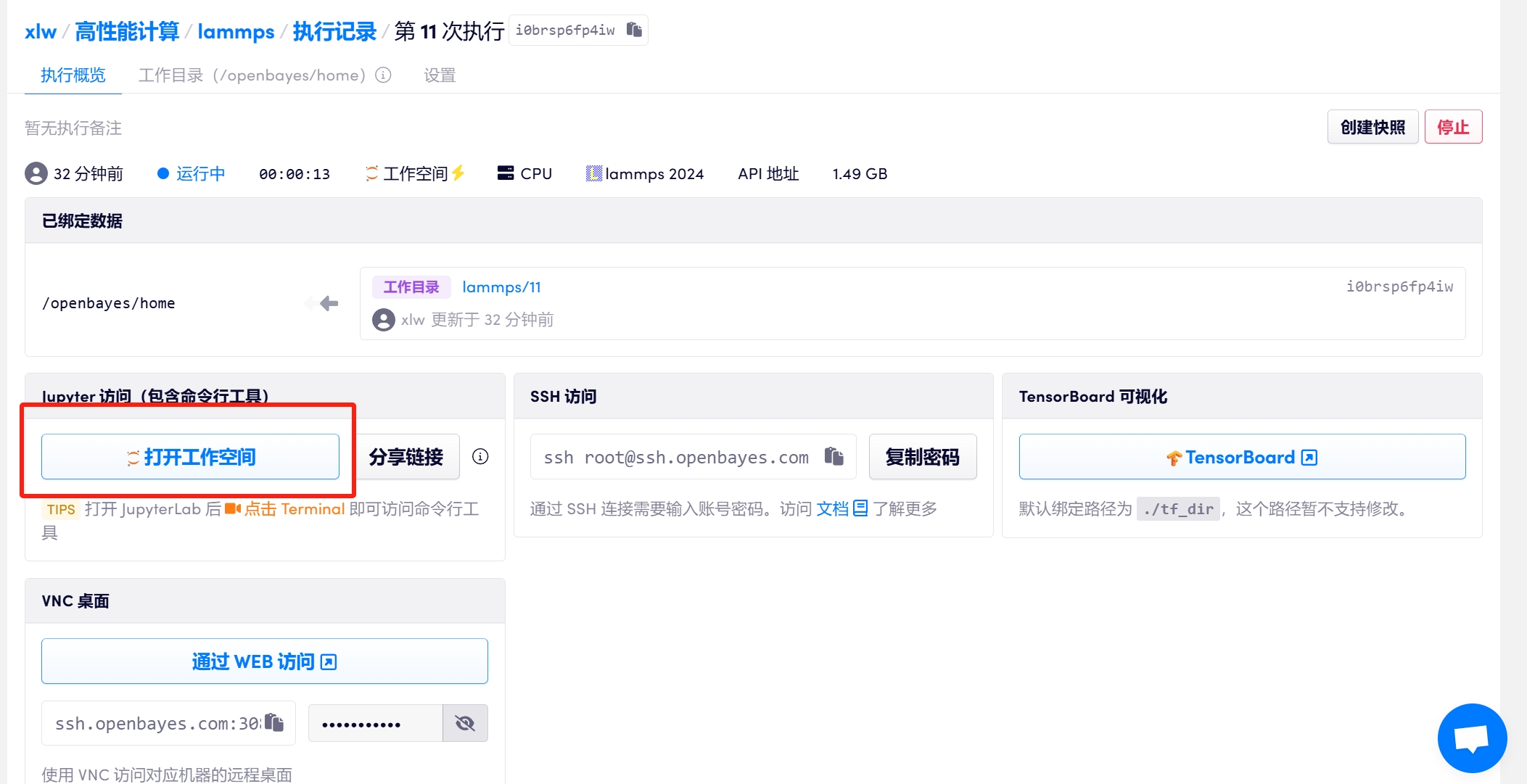
2.1 After the container runs successfully, click on the left to open the workspace
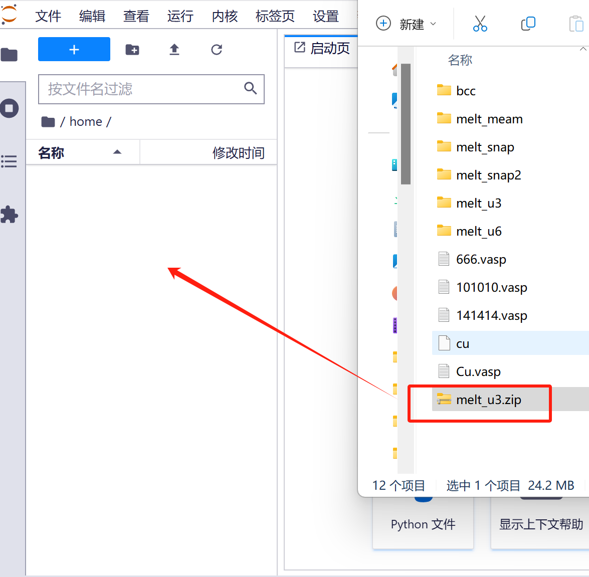
2.2 Drag the compressed package to the file area on the left to upload
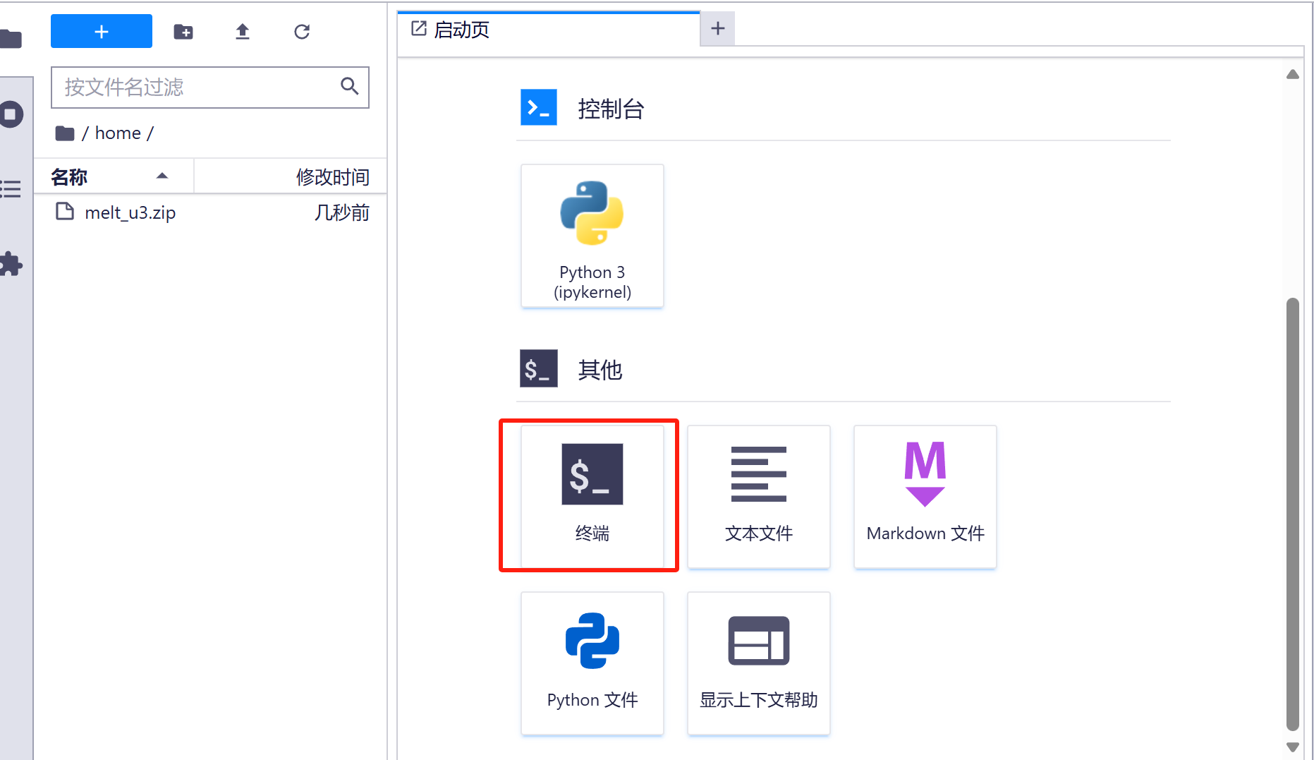
2.3 Then open the terminal
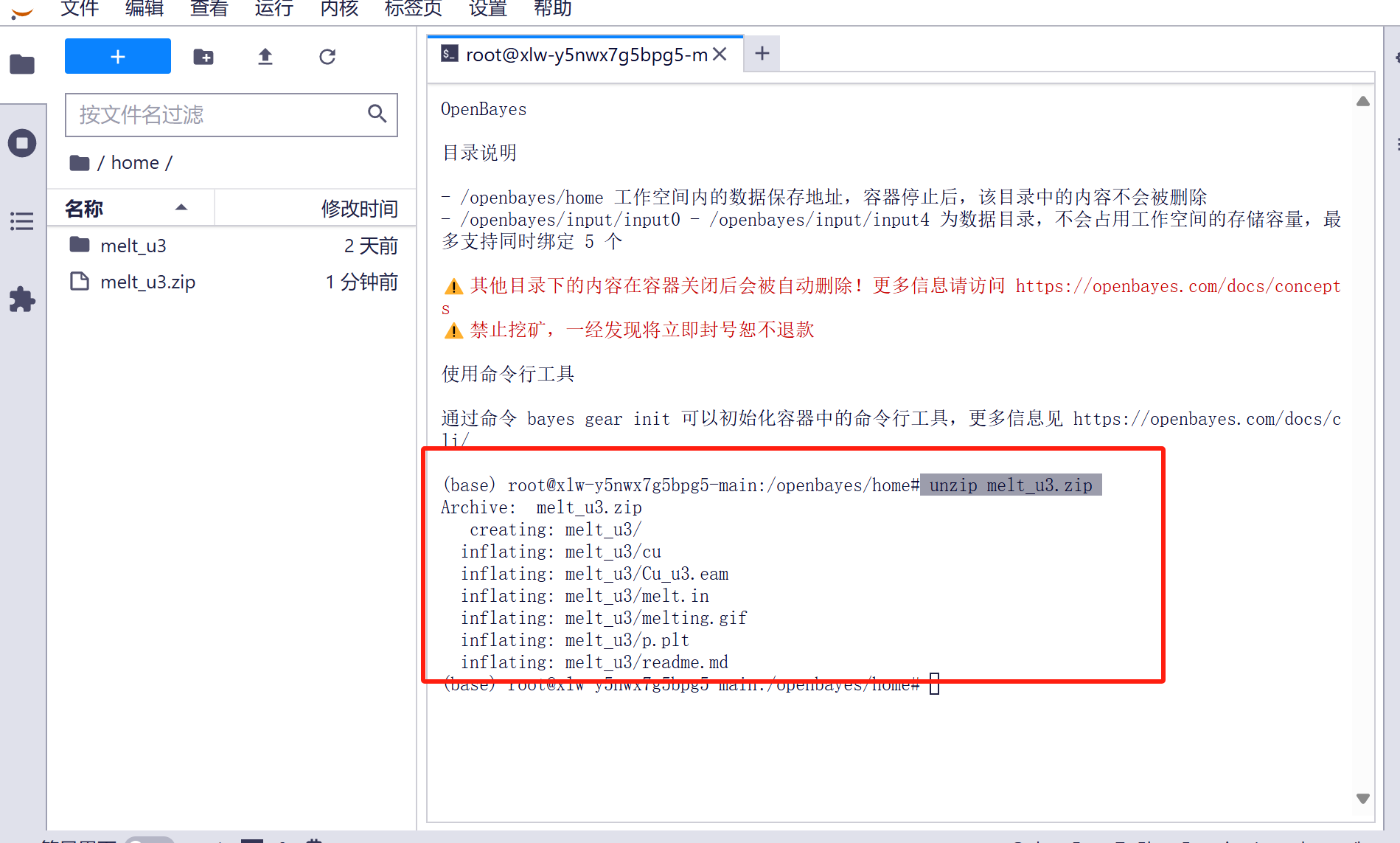
2.4 Unzip (the compressed package has been unzipped in this container, so you can skip this step): Enter unzip melt_u3.zip to unzip the compressed package
unzip melt_u3.zip

Archive:  melt_u3.zip
   creating: melt_u3/
  inflating: melt_u3/cu
  inflating: melt_u3/Cu_u3.eam
  inflating: melt_u3/melt.in
  inflating: melt_u3/melting.gif
  inflating: melt_u3/p.plt
  inflating: melt_u3/readme.md
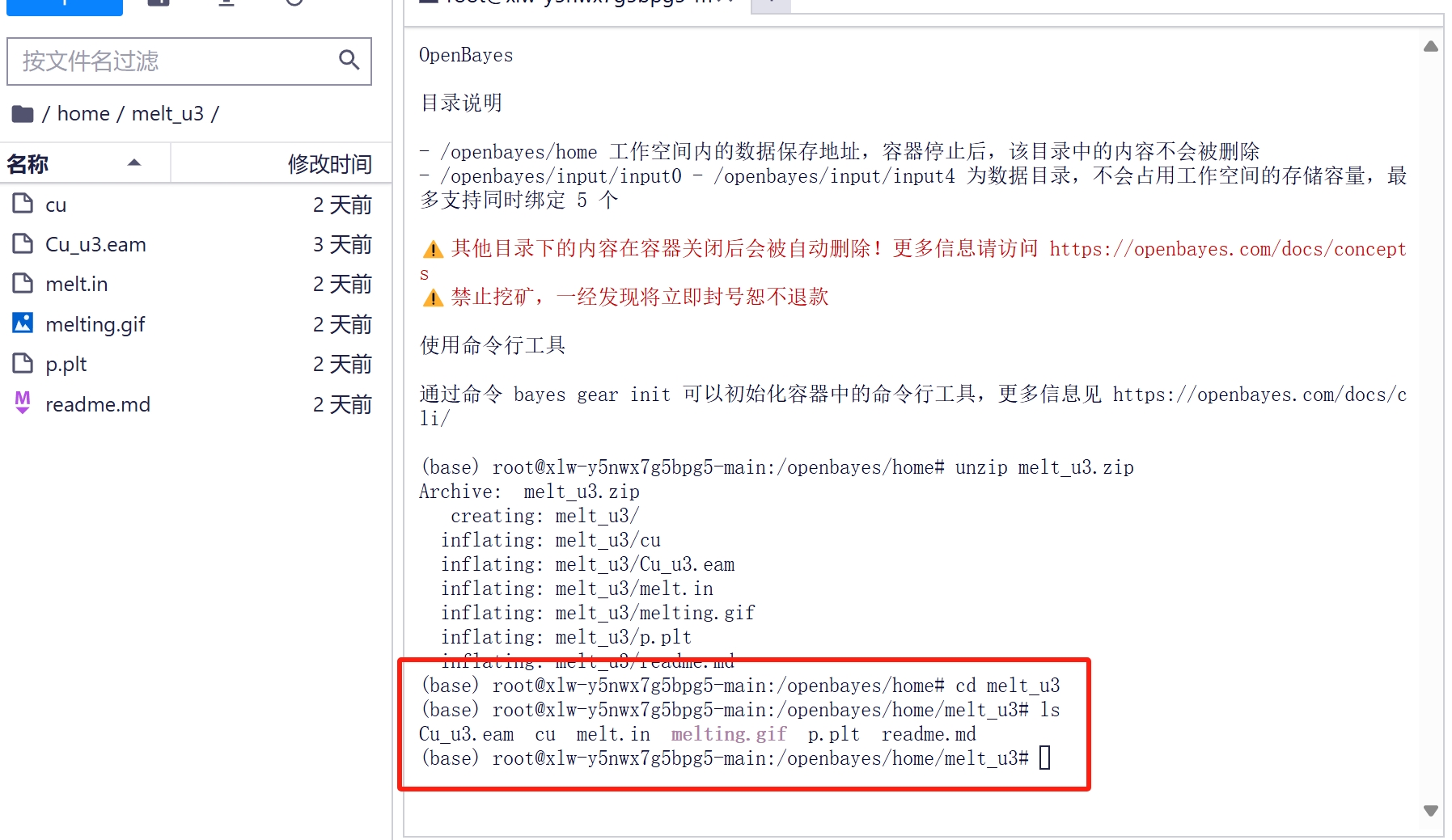
2.5 Enter cd melt_u3 to enter the decompressed directory and use ls to view the files
ls

Cu_u3.eam  cu  melt.in  melting.gif  p.plt  readme.md
2.6 Run lammps
mpirun -np 2 lmp < melt.in | tee out
2.7 The screen output will be synchronized in the out file. The total running time is about 5 minutes.
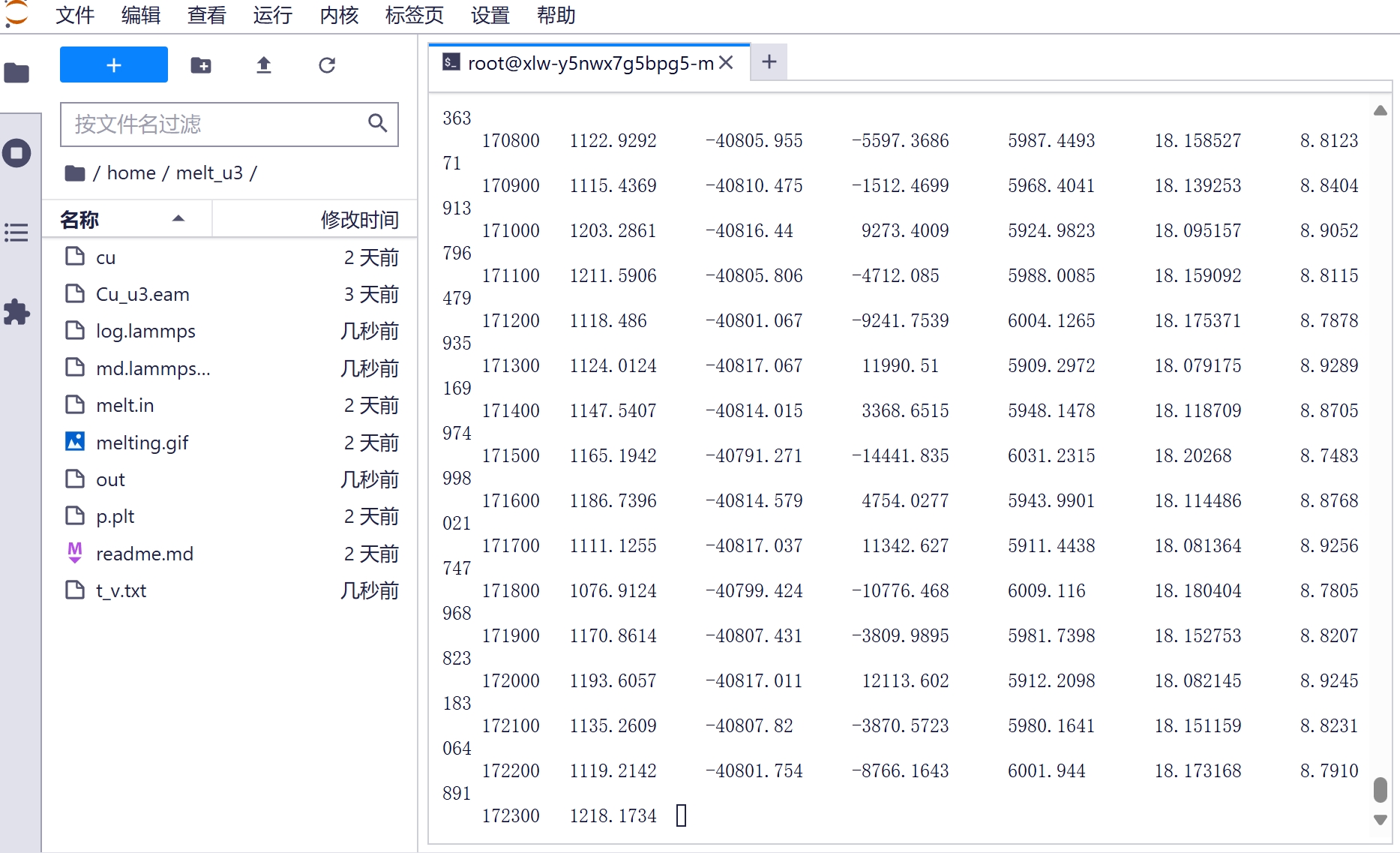
2.8 After the operation is completed, you can get output files such as t_v.txt in the folder
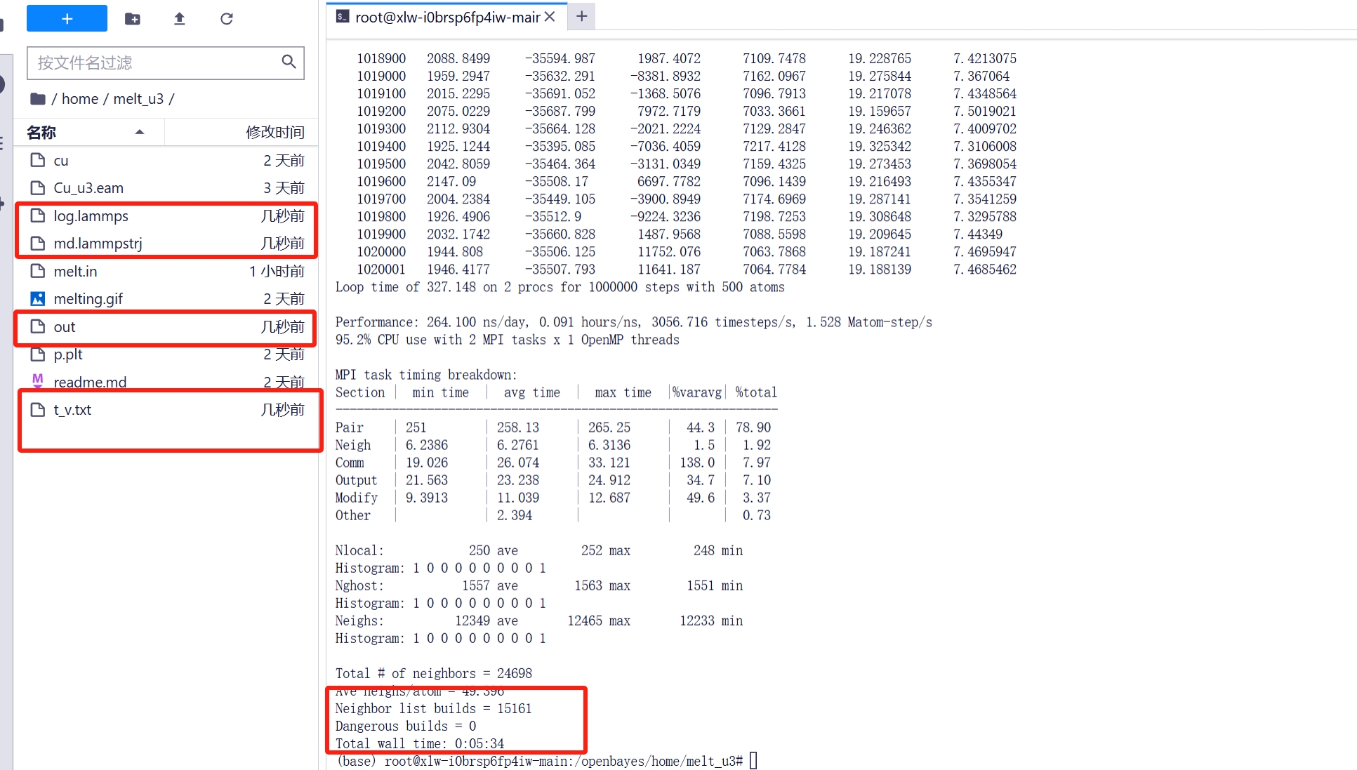
2.9 The t_v.txt file is controlled by the fix command in the input file.
#将温度于体积量分别存储到 t 和 v 中
variable t equal "temp"
variable v equal "vol"

fix                  2 all ave/time 100 10 10000 v_t v_v file t_v.txt
generate
3. Data processing
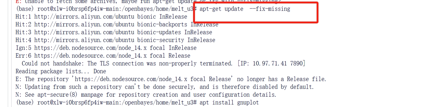
3.1 Update apt source
apt-get update --fix-missing
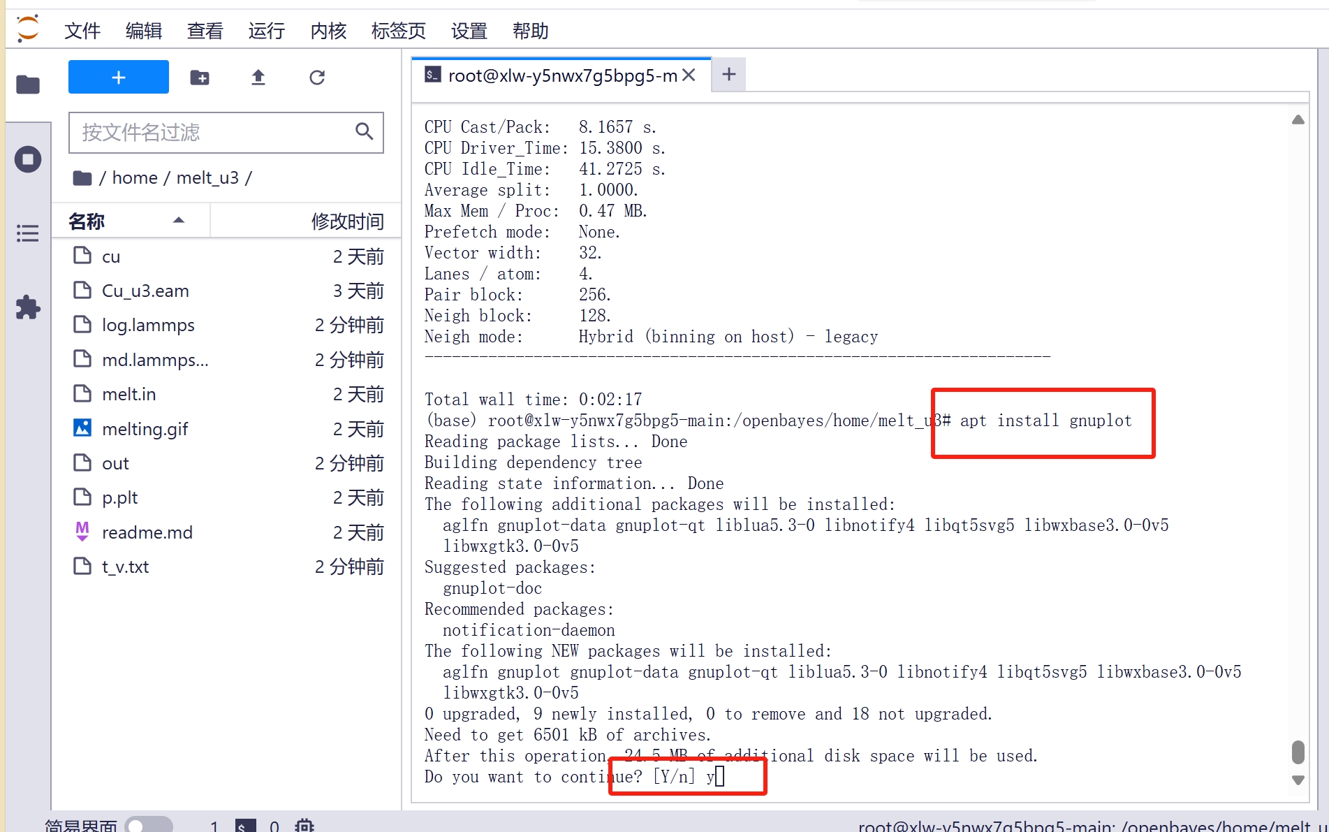
3.2 Type apt install gnuplot to install the gnuplot tool, and then type y and press Enter to confirm.
apt install gnuplot
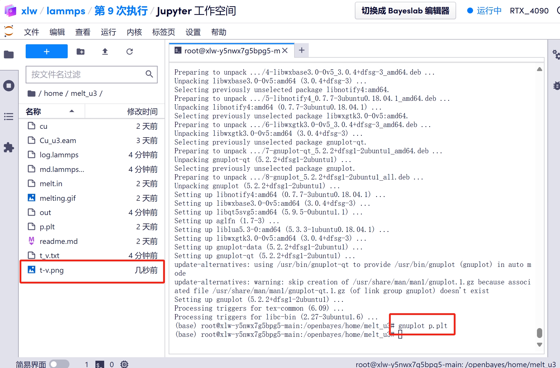
3.3 Run the command gnuplot p.plt to get the tv graph
gnuplot p.plt
3.4 Double-click the left tv graph to get the estimated Cu melting point
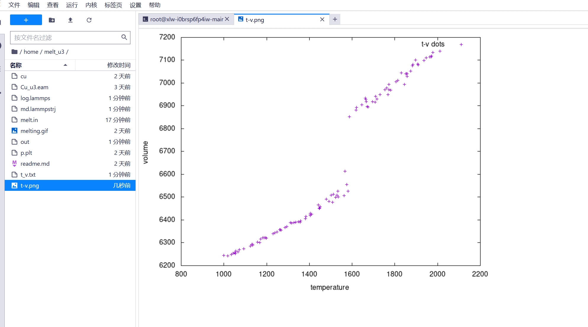
It can be seen that the melting point is around 1600K, which is different from the actual 1357.77K. This is because the temperature rises too quickly and the copper does not have time to melt.
The atomic trajectories during the heating process are given by
#将原子轨迹输出到文件 md.lammpstrj
dump              2 all custom 1 md.lammpstrj id type x y z
Stored in md.lammpstrj, we download it
3.5 Visualization with ovito
Build AI with AI
From idea to launch — accelerate your AI development with free AI co-coding, out-of-the-box environment and best price of GPUs.