Command Palette
Search for a command to run...
GROMACS Getting Started Tutorial: Lysozyme in Water
Date
Molecular dynamics simulation using "lysozyme in water" as an example
Tutorial Introduction
This tutorial is an introductory tutorial on molecular dynamics simulation using GROMACS software. Lysozyme in water As an example learn how to prepare and run a molecular dynamics simulation of a typical protein in water.
The GPU version of GROMACS on the OpenBayes platform, using the NVIDIA RTX 4090 graphics card, has greatly improved its computational efficiency after GPU parallel computing, and the speed can reach 255ns/day! The following is the speed performance:
            Core t (s)   Wall t (s)        (%)
Time:     3972.923      198.659     1999.9
                   (ns/day)    (hour/ns)
Performance:      255.471        0.094
Introduction to GROMACS
GROMACS (GROningen MAchine for Chemical Simulations) is a high-performance software package for molecular dynamics simulations. It is mainly used to model and simulate the motion behavior of biological molecules (such as proteins, lipids and nucleic acids) under different conditions. It was originally developed by the University of Groningen in the Netherlands and has become one of the most commonly used open source tools in the field of molecular dynamics.
Key Features of GROMACS
1. high performance:
• GROMACS is highly optimized for parallel computing and can run efficiently on modern multi-core CPU and GPU systems.
• Supports OpenMP and MPI for multithreaded and distributed computing.
2. Wide range of applications:
• Can be used to simulate the behavior of small molecules to large protein complexes.
• Supports research on biomolecules, polymers, inorganic compounds, and other chemical systems.
3. flexibility:
• Provides a rich set of tools for pre-processing (e.g. topology generation, solvation) and post-processing (e.g. trajectory analysis, energy calculation).
• Support for various force fields, such as AMBER, CHARMM and GROMOS.
4. Ease of use:
• GROMACS includes a user-friendly command line interface.
• Provides detailed documentation and tutorials suitable for both beginners and advanced users.
5. Open source and scalable:
• The open source license allows users to modify and extend GROMACS to suit specific needs.
• Has an active user community and development team.
GROMACS general usage process
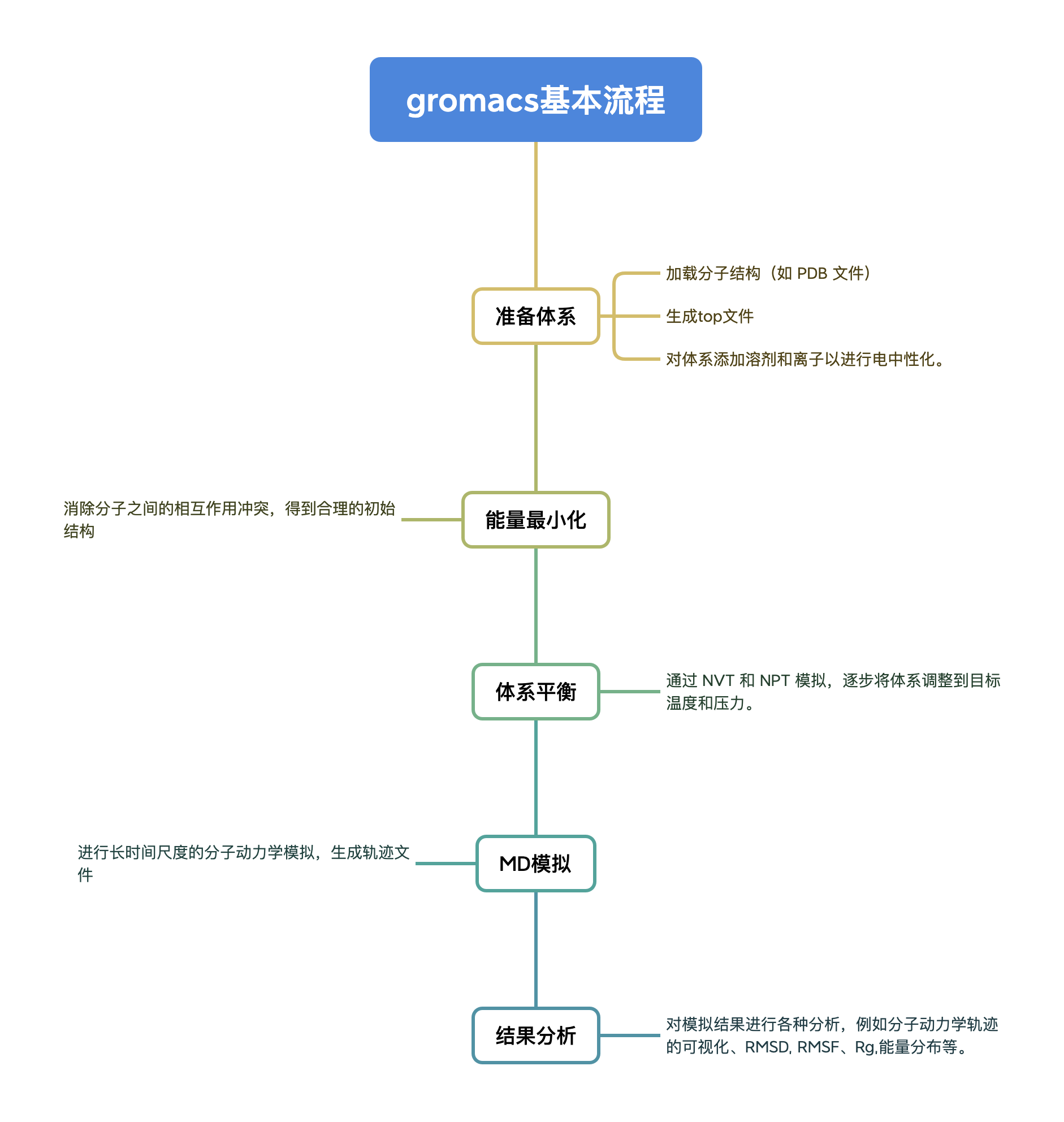
Run steps
First we need to configure the pdb protein file and the md calculation file, and then after various preprocessing, we finally perform a 10ns simulation and analyze the results. The following is a step-by-step explanation.
1. Start GROMACS
首先登录平台:https://openbayes.com/
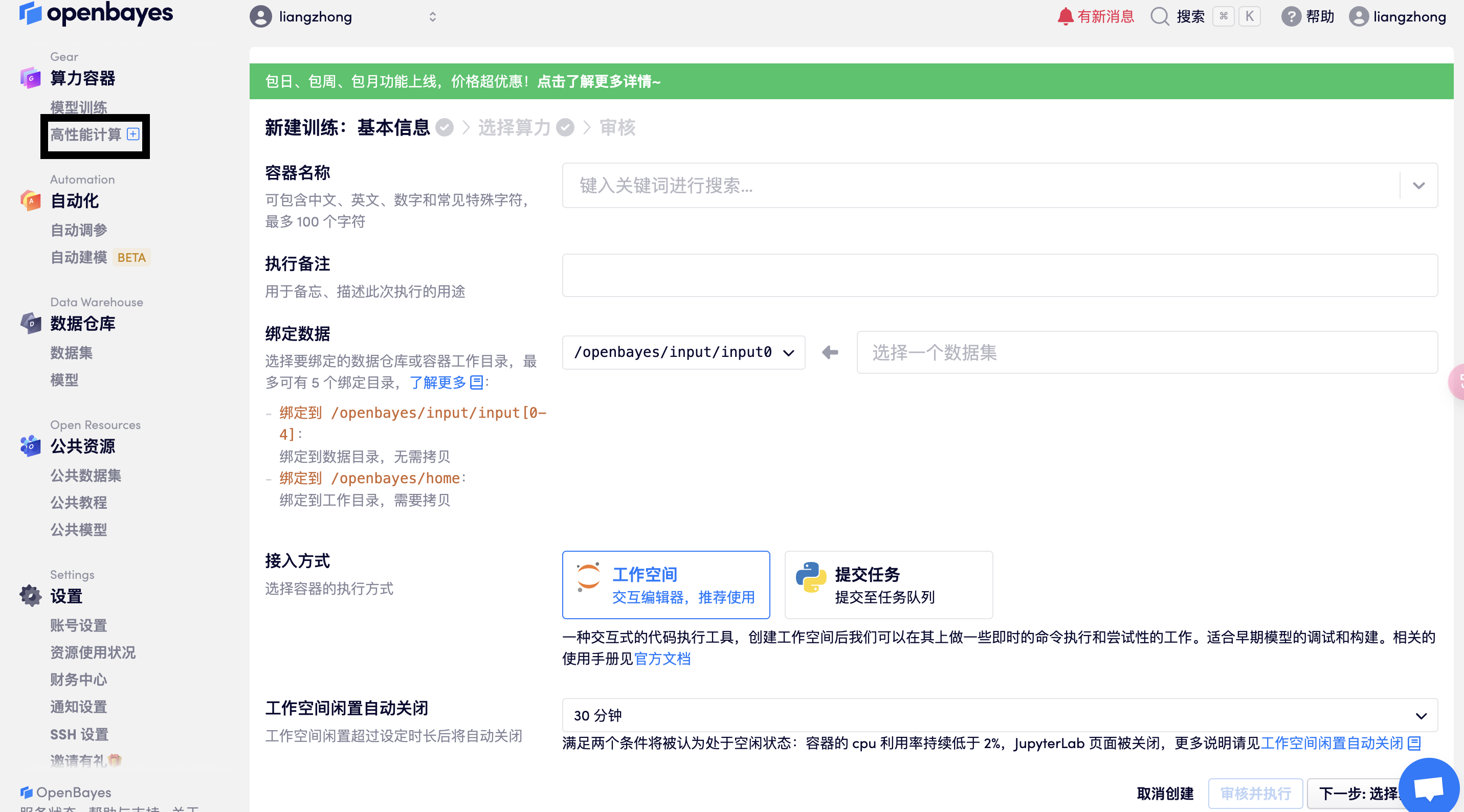
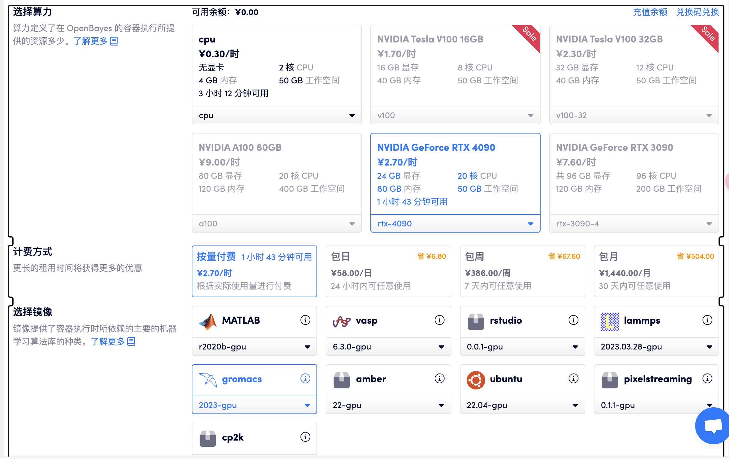
选择「高性能计算」> 创建新容器> 选择算力 RTX 4090> 选择 gromacs GPU
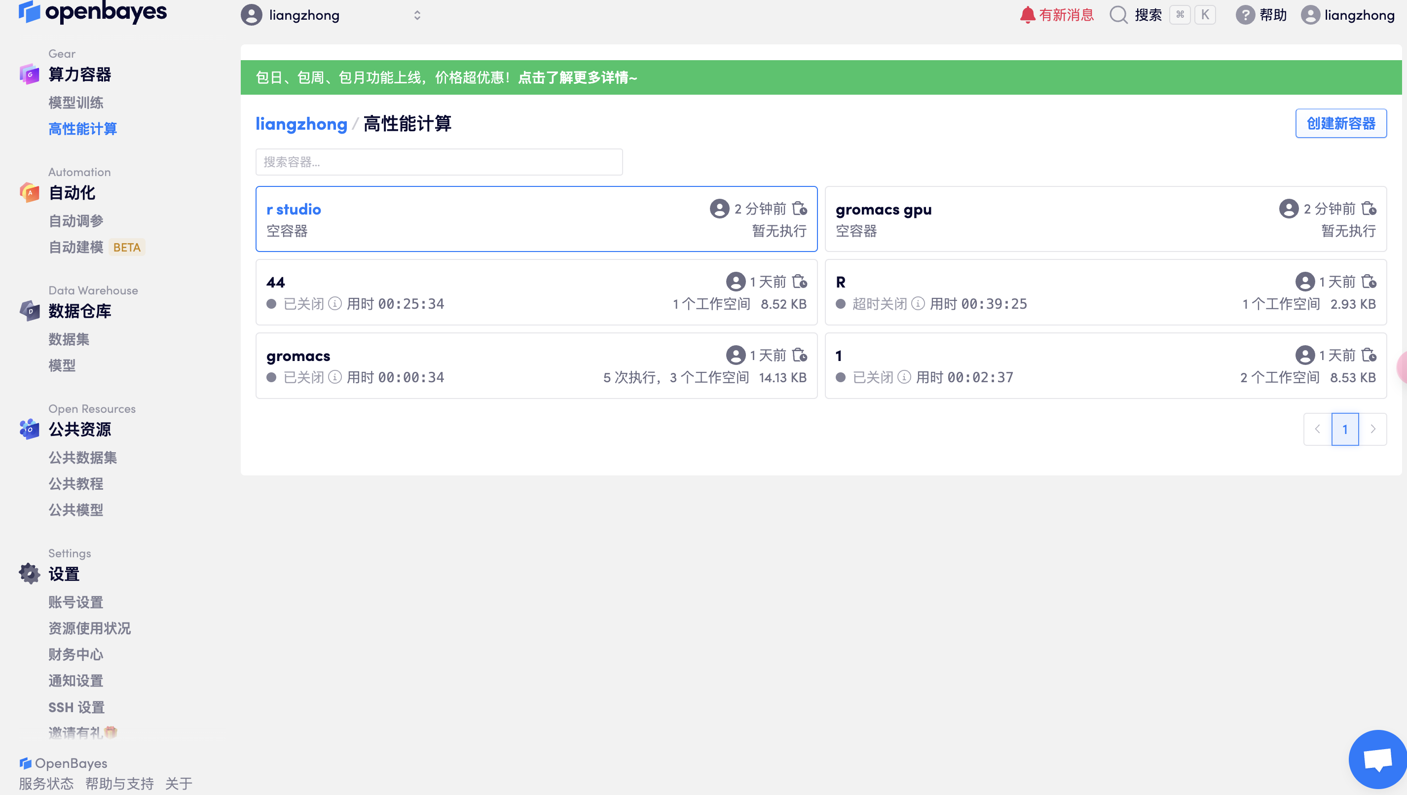
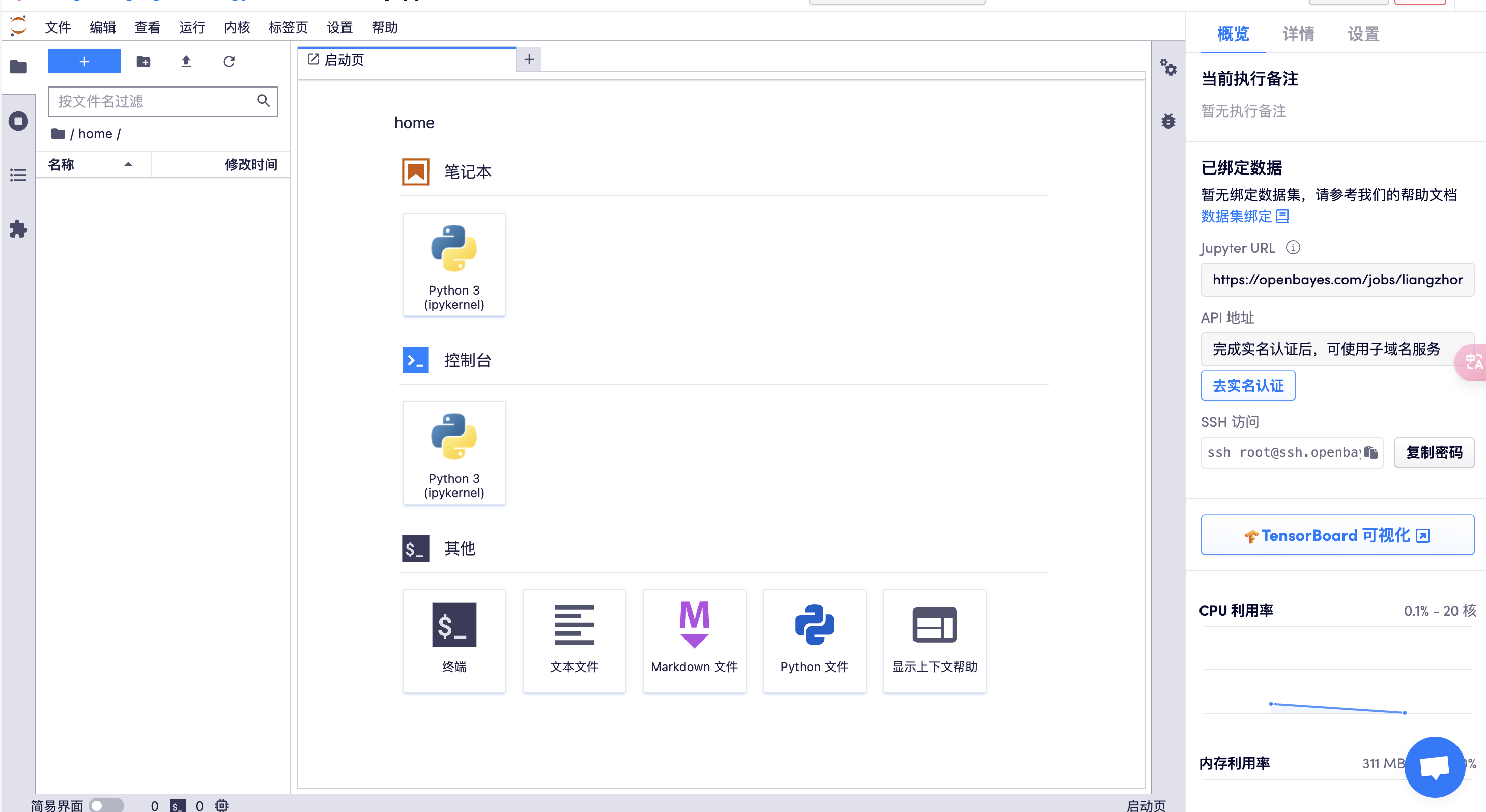
打开工作空间
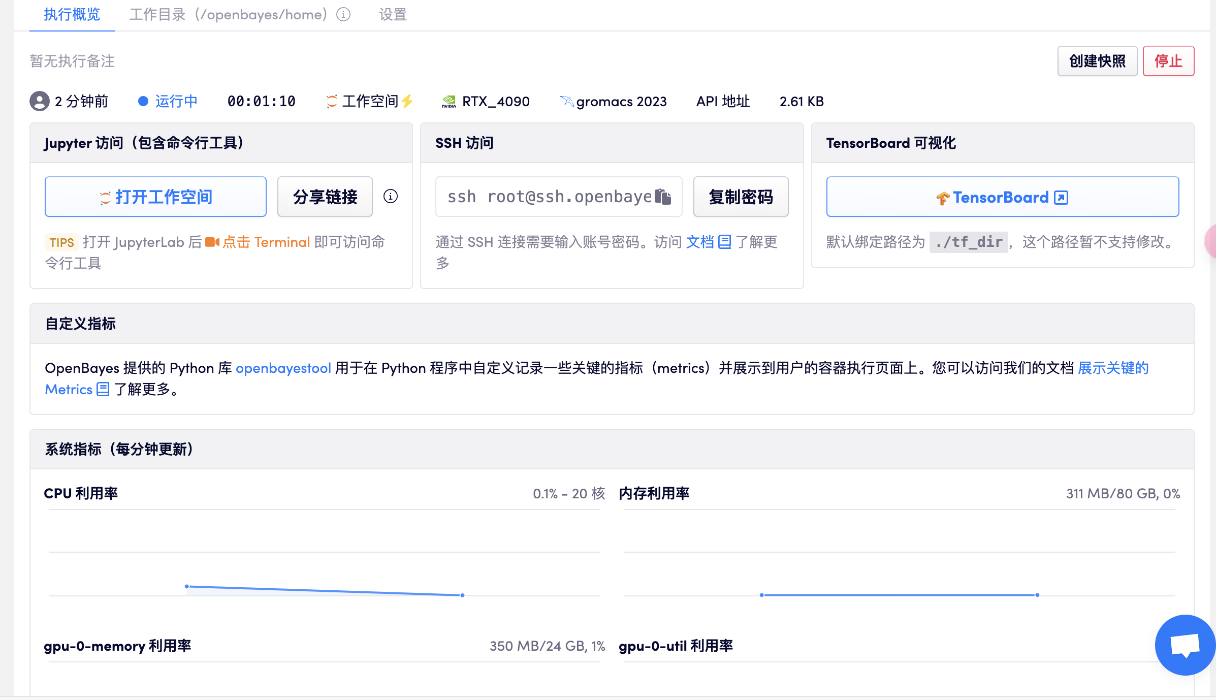
打开终端
或者采用 SSH 控制服务器:

在 X-shell 或者 mac unix 终端,输入:ssh -p 32699  [email protected],再输入密码即可(如下所示)↓
liangzhongzhongzhong@lzr ~ % ssh -p 32699  [email protected]
The authenticity of host '[ssh.openbayes.com]:32699 ([101.237.34.75]:32699)' can't be established.
ED25519 key fingerprint is SHA256:uwPyhP/EYoW49Ez4rvAuaf19czwis2rdS4pImsR0NH8.
This key is not known by any other names.
Are you sure you want to continue connecting (yes/no/[fingerprint])? yes
Warning: Permanently added '[ssh.openbayes.com]:32699' (ED25519) to the list of known hosts.
[email protected]'s password:
OpenBayes

目录说明

- /openbayes/home 工作空间内的数据保存地址,容器停止后,该目录中的内容不会被删除
- /openbayes/input/input0 - /openbayes/input/input4 为数据目录,不会占用工作空间的存储容量,最多支持同时绑定 5 个

⚠️  其他目录下的内容在容器关闭后会被自动删除!更多信息请访问 https://openbayes.com/docs/concepts
⚠️  禁止挖矿,一经发现将立即封号恕不退款

(base) root@liangzhong-4ay9ej85pxvd-main:/openbayes/home# ls
(base) root@liangzhong-4ay9ej85pxvd-main:/openbayes# l(base) root@liangzhong-4ay9ej85pxvd-main:/openbayes# lhome  input  请将文件存在 home 目录下, 当前文件夹下的文件不会被保存.txt
(base) root@liangzhong-4ay9ej85pxvd-main:/openbayes# ls(base) root@liangzhong-4ay9ej85pxvd-main:/openbaye
(base) root@liangzhong-4ay9ej85pxvd-main:/openbayes/input# cd input0
(base) root@liangzhong-4ay9ej85pxvd-main:/openbayes/input/input0# ls
'#nvt.log.1#'    '#topol.top.2#'    1AKI_processed.gro   1aki.pdb   em.log   ions.mdp   mdout.mdp   nvt.cpt   nvt.log   nvt.trr         topol.top
'#nvt.log.2#'     1AKI_clean.pdb    1AKI_solv.gro        em.edr     em.tpr   ions.tpr   minim.mdp   nvt.edr   nvt.mdp   posre.itp
'#topol.top.1#'   1AKI_newbox.gro   1AKI_solv_ions.gro   em.gro     em.trr   md.mdp     npt.mdp     nvt.gro   nvt.tpr   potential.xvg
(base) root@liangzhong-4ay9ej85pxvd-main:/openbayes/input/input0#

调用 GROMACS,设置临时环境变量
export PATH=/data/app/gromacs/bin:$PATH
(base) root@liangzhong-4ay9ej85pxvd-main:/openbayes/home# gmx_mpi -h
                        :-) GROMACS - gmx_mpi, 2023 (-:

Executable:   /data/app/gromacs/bin/gmx_mpi
Data prefix:  /data/app/gromacs
Working dir:  /output
Command line:
  gmx_mpi -h

SYNOPSIS

gmx [-[no]h] [-[no]quiet] [-[no]version] [-[no]copyright] [-nice <int>]
    [-[no]backup]

OPTIONS

Other options:

 -[no]h                     (no)
           Print help and quit
 -[no]quiet                 (no)
           Do not print common startup info or quotes
 -[no]version               (no)
           Print extended version information and quit
 -[no]copyright             (no)
           Print copyright information on startup
 -nice   <int>              (19)
           Set the nicelevel (default depends on command)
 -[no]backup                (yes)
           Write backups if output files exist

Additional help is available on the following topics:
    commands    List of available commands
    selections  Selection syntax and usage
To access the help, use 'gmx help <topic>'.
For help on a command, use 'gmx help <command>'.

GROMACS reminds you: "All You Need is Greed" (Aztec Camera)
2. Document preparation
Before running the tutorial, we need to prepare the following 6 files: 1aki.pdb, ions.mdp, md.mdp, minim.mdp, npt.mdp, nvt.mdp
These files can be downloaded directly, or created as follows.
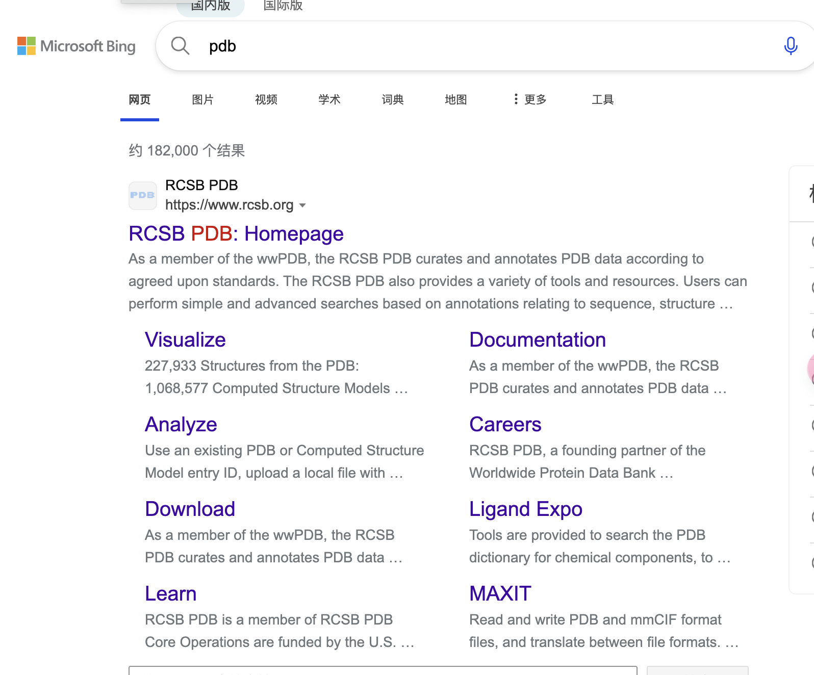
For example, 1AKI.pdb protein file: can be obtained from RCSB Get 1AKI.pdb from the website.In the tutorial, other files have been created by copying the code using the vim text editor.
RCSB Database Introduction:
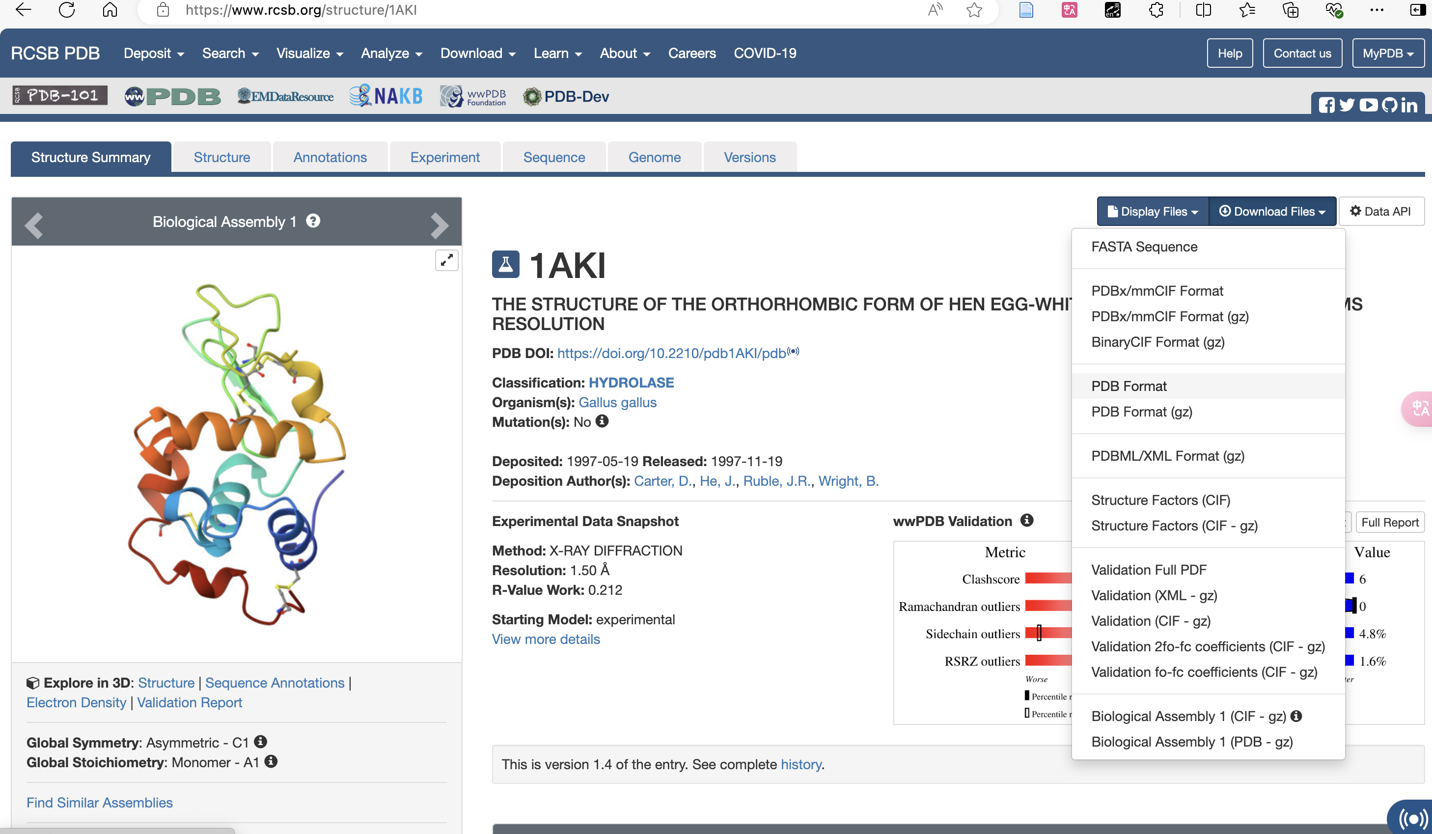
Download pdb Format:
Upload to your working directory
(base) root@liangzhong-4ay9ej85pxvd-main:/input0# ls
1aki.pdb
#查看上传成功
vim ions.mdp
#准备 mdp 文件,输入命令后复制一下内容,按 i 进入插入模式开始编辑。
#编辑完成后,按 Esc 键退出插入模式,输入 :wq 保存并退出。
; ions.mdp - used as input into grompp to generate ions.tpr
; Parameters describing what to do, when to stop and what to save
integrator  = steep         ; Algorithm (steep = steepest descent minimization)
emtol       = 1000.0        ; Stop minimization when the maximum force < 1000.0 kJ/mol/nm
emstep      = 0.01          ; Minimization step size
nsteps      = 50000         ; Maximum number of (minimization) steps to perform

; Parameters describing how to find the neighbors of each atom and how to calculate the interactions
nstlist         = 1         ; Frequency to update the neighbor list and long range forces
cutoff-scheme	= Verlet    ; Buffered neighbor searching
ns_type         = grid      ; Method to determine neighbor list (simple, grid)
coulombtype     = cutoff    ; Treatment of long range electrostatic interactions
rcoulomb        = 1.0       ; Short-range electrostatic cut-off
rvdw            = 1.0       ; Short-range Van der Waals cut-off
pbc             = xyz       ; Periodic Boundary Conditions in all 3 dimensions
vim minim.mdp

; minim.mdp - used as input into grompp to generate em.tpr
; Parameters describing what to do, when to stop and what to save
integrator  = steep         ; Algorithm (steep = steepest descent minimization)
emtol       = 1000.0        ; Stop minimization when the maximum force < 1000.0 kJ/mol/nm
emstep      = 0.01          ; Minimization step size
nsteps      = 50000         ; Maximum number of (minimization) steps to perform

; Parameters describing how to find the neighbors of each atom and how to calculate the interactions
nstlist         = 1         ; Frequency to update the neighbor list and long range forces
cutoff-scheme   = Verlet    ; Buffered neighbor searching
ns_type         = grid      ; Method to determine neighbor list (simple, grid)
coulombtype     = PME       ; Treatment of long range electrostatic interactions
rcoulomb        = 1.0       ; Short-range electrostatic cut-off
rvdw            = 1.0       ; Short-range Van der Waals cut-off
pbc             = xyz       ; Periodic Boundary Conditions in all 3 dimensions
vim nvt.mdp

title                   = OPLS Lysozyme NVT equilibration
define                  = -DPOSRES  ; position restrain the protein
; Run parameters
integrator              = md        ; leap-frog integrator
nsteps                  = 50000     ; 2 * 50000 = 100 ps
dt                      = 0.002     ; 2 fs
; Output control
nstxout                 = 500       ; save coordinates every 1.0 ps
nstvout                 = 500       ; save velocities every 1.0 ps
nstenergy               = 500       ; save energies every 1.0 ps
nstlog                  = 500       ; update log file every 1.0 ps
; Bond parameters
continuation            = no        ; first dynamics run
constraint_algorithm    = lincs     ; holonomic constraints
constraints             = h-bonds   ; bonds involving H are constrained
lincs_iter              = 1         ; accuracy of LINCS
lincs_order             = 4         ; also related to accuracy
; Nonbonded settings
cutoff-scheme           = Verlet    ; Buffered neighbor searching
ns_type                 = grid      ; search neighboring grid cells
nstlist                 = 10        ; 20 fs, largely irrelevant with Verlet
rcoulomb                = 1.0       ; short-range electrostatic cutoff (in nm)
rvdw                    = 1.0       ; short-range van der Waals cutoff (in nm)
DispCorr                = EnerPres  ; account for cut-off vdW scheme
; Electrostatics
coulombtype             = PME       ; Particle Mesh Ewald for long-range electrostatics
pme_order               = 4         ; cubic interpolation
fourierspacing          = 0.16      ; grid spacing for FFT
; Temperature coupling is on
tcoupl                  = V-rescale             ; modified Berendsen thermostat
tc-grps                 = Protein Non-Protein   ; two coupling groups - more accurate
tau_t                   = 0.1     0.1           ; time constant, in ps
ref_t                   = 300     300           ; reference temperature, one for each group, in K
; Pressure coupling is off
pcoupl                  = no        ; no pressure coupling in NVT
; Periodic boundary conditions
pbc                     = xyz       ; 3-D PBC
; Velocity generation
gen_vel                 = yes       ; assign velocities from Maxwell distribution
gen_temp                = 300       ; temperature for Maxwell distribution
gen_seed                = -1        ; generate a random seed
vim npt.mdp

title                   = OPLS Lysozyme NPT equilibration
define                  = -DPOSRES  ; position restrain the protein
; Run parameters
integrator              = md        ; leap-frog integrator
nsteps                  = 50000     ; 2 * 50000 = 100 ps
dt                      = 0.002     ; 2 fs
; Output control
nstxout                 = 500       ; save coordinates every 1.0 ps
nstvout                 = 500       ; save velocities every 1.0 ps
nstenergy               = 500       ; save energies every 1.0 ps
nstlog                  = 500       ; update log file every 1.0 ps
; Bond parameters
continuation            = yes       ; Restarting after NVT
constraint_algorithm    = lincs     ; holonomic constraints
constraints             = h-bonds   ; bonds involving H are constrained
lincs_iter              = 1         ; accuracy of LINCS
lincs_order             = 4         ; also related to accuracy
; Nonbonded settings
cutoff-scheme           = Verlet    ; Buffered neighbor searching
ns_type                 = grid      ; search neighboring grid cells
nstlist                 = 10        ; 20 fs, largely irrelevant with Verlet scheme
rcoulomb                = 1.0       ; short-range electrostatic cutoff (in nm)
rvdw                    = 1.0       ; short-range van der Waals cutoff (in nm)
DispCorr                = EnerPres  ; account for cut-off vdW scheme
; Electrostatics
coulombtype             = PME       ; Particle Mesh Ewald for long-range electrostatics
pme_order               = 4         ; cubic interpolation
fourierspacing          = 0.16      ; grid spacing for FFT
; Temperature coupling is on
tcoupl                  = V-rescale             ; modified Berendsen thermostat
tc-grps                 = Protein Non-Protein   ; two coupling groups - more accurate
tau_t                   = 0.1     0.1           ; time constant, in ps
ref_t                   = 300     300           ; reference temperature, one for each group, in K
; Pressure coupling is on
pcoupl                  = Parrinello-Rahman     ; Pressure coupling on in NPT
pcoupltype              = isotropic             ; uniform scaling of box vectors
tau_p                   = 2.0                   ; time constant, in ps
ref_p                   = 1.0                   ; reference pressure, in bar
compressibility         = 4.5e-5                ; isothermal compressibility of water, bar^-1
refcoord_scaling        = com
; Periodic boundary conditions
pbc                     = xyz       ; 3-D PBC
; Velocity generation
gen_vel                 = no        ; Velocity generation is off
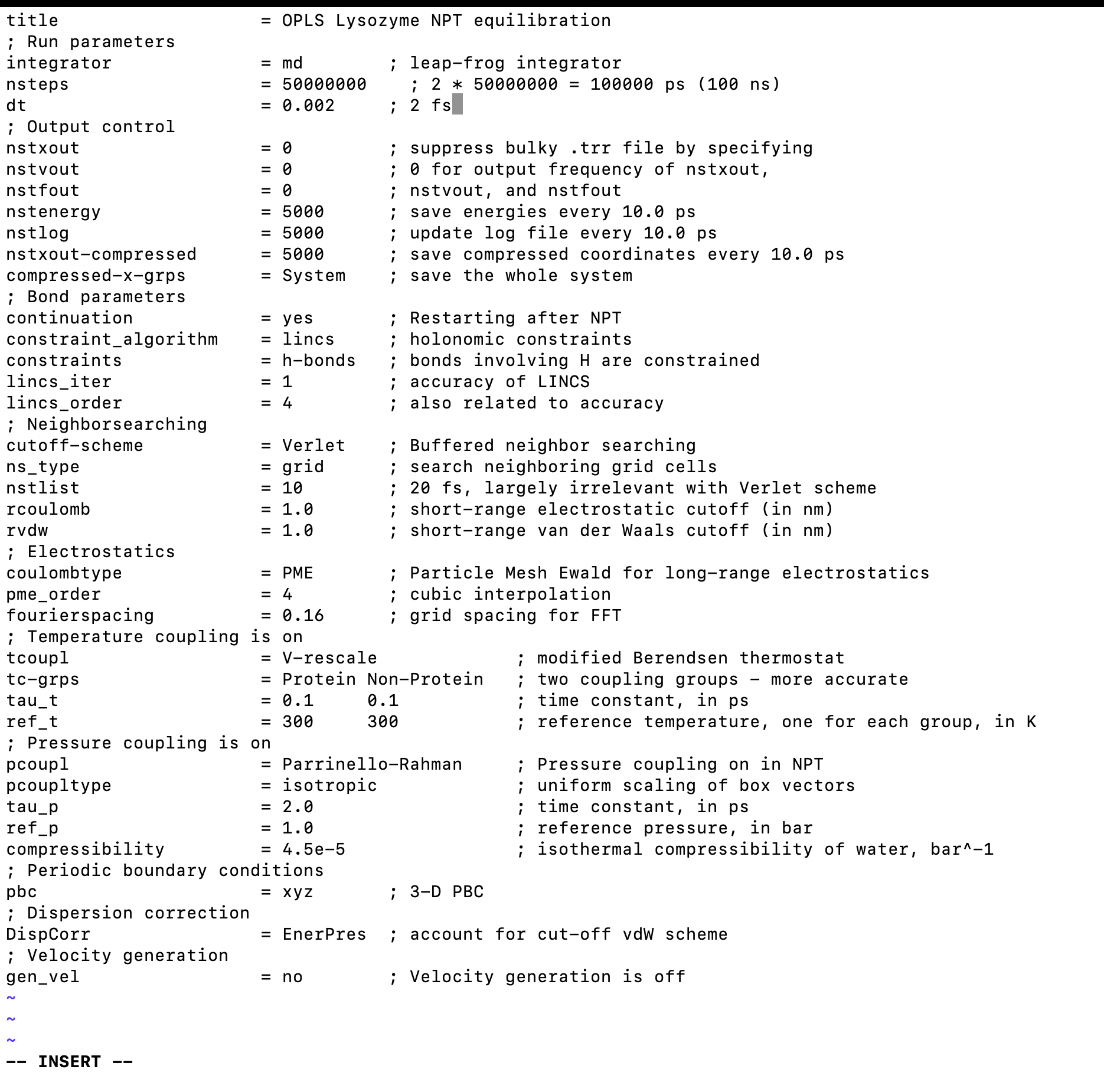
vim md.md

title                   = OPLS Lysozyme NPT equilibration
; Run parameters
integrator              = md        ; leap-frog integrator
nsteps                  = 500000    ; 2 * 500000 = 1000 ps (1 ns)
dt                      = 0.002     ; 2 fs
; Output control
nstxout                 = 0         ; suppress bulky .trr file by specifying
nstvout                 = 0         ; 0 for output frequency of nstxout,
nstfout                 = 0         ; nstvout, and nstfout
nstenergy               = 5000      ; save energies every 10.0 ps
nstlog                  = 5000      ; update log file every 10.0 ps
nstxout-compressed      = 5000      ; save compressed coordinates every 10.0 ps
compressed-x-grps       = System    ; save the whole system
; Bond parameters
continuation            = yes       ; Restarting after NPT
constraint_algorithm    = lincs     ; holonomic constraints
constraints             = h-bonds   ; bonds involving H are constrained
lincs_iter              = 1         ; accuracy of LINCS
lincs_order             = 4         ; also related to accuracy
; Neighborsearching
cutoff-scheme           = Verlet    ; Buffered neighbor searching
ns_type                 = grid      ; search neighboring grid cells
nstlist                 = 10        ; 20 fs, largely irrelevant with Verlet scheme
rcoulomb                = 1.0       ; short-range electrostatic cutoff (in nm)
rvdw                    = 1.0       ; short-range van der Waals cutoff (in nm)
; Electrostatics
coulombtype             = PME       ; Particle Mesh Ewald for long-range electrostatics
pme_order               = 4         ; cubic interpolation
fourierspacing          = 0.16      ; grid spacing for FFT
; Temperature coupling is on
tcoupl                  = V-rescale             ; modified Berendsen thermostat
tc-grps                 = Protein Non-Protein   ; two coupling groups - more accurate
tau_t                   = 0.1     0.1           ; time constant, in ps
ref_t                   = 300     300           ; reference temperature, one for each group, in K
; Pressure coupling is on
pcoupl                  = Parrinello-Rahman     ; Pressure coupling on in NPT
pcoupltype              = isotropic             ; uniform scaling of box vectors
tau_p                   = 2.0                   ; time constant, in ps
ref_p                   = 1.0                   ; reference pressure, in bar
compressibility         = 4.5e-5                ; isothermal compressibility of water, bar^-1
; Periodic boundary conditions
pbc                     = xyz       ; 3-D PBC
; Dispersion correction
DispCorr                = EnerPres  ; account for cut-off vdW scheme
; Velocity generation
gen_vel                 = no        ; Velocity generation is off
2. Formal simulation steps
Target: Build a physically reasonable simulation system to lay the foundation for subsequent dynamic simulation.
1. Load molecular structure (PDB file):
• PDB Files(Protein Data Bank) contains three-dimensional coordinates and structural information of molecules (such as proteins, nucleic acids, and small molecules).
• GROMACS uses the pdb2gmx tool to convert this coordinate information into a molecular model and assign force field parameters.
• Force Field: A mathematical model that describes the interactions between molecules, including bonds, angles, dihedral potential energy, van der Waals forces, and charge interactions.
• Common force fields: GROMOS, AMBER, CHARMM.
(Commonly used ones are AMBER99SB protein, OPLS-AA/L all-atom force field, charm36 force field (need to download and configure by yourself), other force fields are too old and not suitable for publishing articles)
2. Generate topology file:
• The topology file (topol.top) defines the force field parameters of each molecule in the simulation system, such as atom type, bond type and its parameters, etc.
• It combines with the coordinate file to form the basis of molecular dynamics simulations.
3. Run pdb2gmx, select force field: 15 and press Enter
#删除水分子(PDB 文件中的 “HOH” 残基)
grep -v HOH 1aki.pdb > 1AKI_clean.pdb
gmx_mpi pdb2gmx -f 1AKI_clean.pdb -o 1AKI_processed.gro -water spce
#选择 15,按回车,OPLS-AA/L all-atom force field (2001 aminoacid dihedrals)

(base) root@liangzhong-4ay9ej85pxvd-main:/input0#  pdb2gmx -f 1AKI_clean.pdb -o 1AKI_processed.gro -water spce
                      :-) GROMACS - gmx pdb2gmx, 2023 (-:

Executable:   /data/app/gromacs/bin/gmx_mpi
Data prefix:  /data/app/gromacs
Working dir:  /input0
Command line:
  gmx_mpi pdb2gmx -f 1AKI_clean.pdb -o 1AKI_processed.gro -water spce

Select the Force Field:

From '/data/app/gromacs/share/gromacs/top':

 1: AMBER03 protein, nucleic AMBER94 (Duan et al., J. Comp. Chem. 24, 1999-2012, 2003)

 2: AMBER94 force field (Cornell et al., JACS 117, 5179-5197, 1995)

 3: AMBER96 protein, nucleic AMBER94 (Kollman et al., Acc. Chem. Res. 29, 461-469, 1996)

 4: AMBER99 protein, nucleic AMBER94 (Wang et al., J. Comp. Chem. 21, 1049-1074, 2000)

 5: AMBER99SB protein, nucleic AMBER94 (Hornak et al., Proteins 65, 712-725, 2006)

 6: AMBER99SB-ILDN protein, nucleic AMBER94 (Lindorff-Larsen et al., Proteins 78, 1950-58, 2010)

 7: AMBERGS force field (Garcia & Sanbonmatsu, PNAS 99, 2782-2787, 2002)

 8: CHARMM27 all-atom force field (CHARM22 plus CMAP for proteins)

 9: GROMOS96 43a1 force field

10: GROMOS96 43a2 force field (improved alkane dihedrals)

11: GROMOS96 45a3 force field (Schuler JCC 2001 22 1205)

12: GROMOS96 53a5 force field (JCC 2004 vol 25 pag 1656)

13: GROMOS96 53a6 force field (JCC 2004 vol 25 pag 1656)

14: GROMOS96 54a7 force field (Eur. Biophys. J. (2011), 40,, 843-856, DOI: 10.1007/s00249-011-0700-9)

15: OPLS-AA/L all-atom force field (2001 aminoacid dihedrals)
15

Using the Oplsaa force field in directory oplsaa.ff

going to rename oplsaa.ff/aminoacids.r2b
Opening force field file /data/app/gromacs/share/gromacs/top/oplsaa.ff/aminoacids.r2b
Reading 1AKI_clean.pdb...
WARNING: all CONECT records are ignored
Read 'LYSOZYME', 1001 atoms

Analyzing pdb file
Splitting chemical chains based on TER records or chain id changing.

There are 1 chains and 0 blocks of water and 129 residues with 1001 atoms

  chain  #res #atoms

  1 'A'   129   1001

All occupancies are one
All occupancies are one
Opening force field file /data/app/gromacs/share/gromacs/top/oplsaa.ff/atomtypes.atp

Reading residue database... (Oplsaa)
Opening force field file /data/app/gromacs/share/gromacs/top/oplsaa.ff/aminoacids.rtp
Opening force field file /data/app/gromacs/share/gromacs/top/oplsaa.ff/aminoacids.hdb
Opening force field file /data/app/gromacs/share/gromacs/top/oplsaa.ff/aminoacids.n.tdb
Opening force field file /data/app/gromacs/share/gromacs/top/oplsaa.ff/aminoacids.c.tdb

Processing chain 1 'A' (1001 atoms, 129 residues)
Analysing hydrogen-bonding network for automated assignment of histidine
 protonation. 213 donors and 184 acceptors were found.
There are 255 hydrogen bonds
Will use HISE for residue 15

Identified residue LYS1 as a starting terminus.

Identified residue LEU129 as a ending terminus.
8 out of 8 lines of specbond.dat converted successfully
Special Atom Distance matrix:
                    CYS6   MET12   HIS15   CYS30   CYS64   CYS76   CYS80
                    SG48    SD87  NE2118   SG238   SG513   SG601   SG630
   MET12    SD87   1.166
   HIS15  NE2118   1.776   1.019
   CYS30   SG238   1.406   1.054   2.069
   CYS64   SG513   2.835   1.794   1.789   2.241
   CYS76   SG601   2.704   1.551   1.468   2.116   0.765
   CYS80   SG630   2.959   1.951   1.916   2.391   0.199   0.944
   CYS94   SG724   2.550   1.407   1.382   1.975   0.665   0.202   0.855
  MET105   SD799   1.827   0.911   1.683   0.888   1.849   1.461   2.036
  CYS115   SG889   1.576   1.084   2.078   0.200   2.111   1.989   2.262
  CYS127   SG981   0.197   1.072   1.721   1.313   2.799   2.622   2.934
                   CYS94  MET105  CYS115
                   SG724   SD799   SG889
  MET105   SD799   1.381
  CYS115   SG889   1.853   0.790
  CYS127   SG981   2.475   1.686   1.483
Linking CYS-6 SG-48 and CYS-127 SG-981...
Linking CYS-30 SG-238 and CYS-115 SG-889...
Linking CYS-64 SG-513 and CYS-80 SG-630...
Linking CYS-76 SG-601 and CYS-94 SG-724...
Start terminus LYS-1: NH3+
End terminus LEU-129: COO-

Checking for duplicate atoms....

Generating any missing hydrogen atoms and/or adding termini.

Now there are 129 residues with 1960 atoms

Making bonds...

Number of bonds was 1984, now 1984

Generating angles, dihedrals and pairs...
Before cleaning: 5142 pairs
Before cleaning: 5187 dihedrals

Making cmap torsions...

There are 5187 dihedrals,  426 impropers, 3547 angles
          5106 pairs,     1984 bonds and     0 virtual sites

Total mass 14313.193 a.m.u.

Total charge 8.000 e

Writing topology

Writing coordinate file...

                --------- PLEASE NOTE ------------

You have successfully generated a topology from: 1AKI_clean.pdb.

The Oplsaa force field and the spce water model are used.

                --------- ETON ESAELP ------------

GROMACS reminds you: "Any one who considers arithmetical methods of producing random digits is, of course, in a state of sin." (John von Neumann)
You can see that there are several more files, and "Total charge 8.000 e" We will need to neutralize the charge later
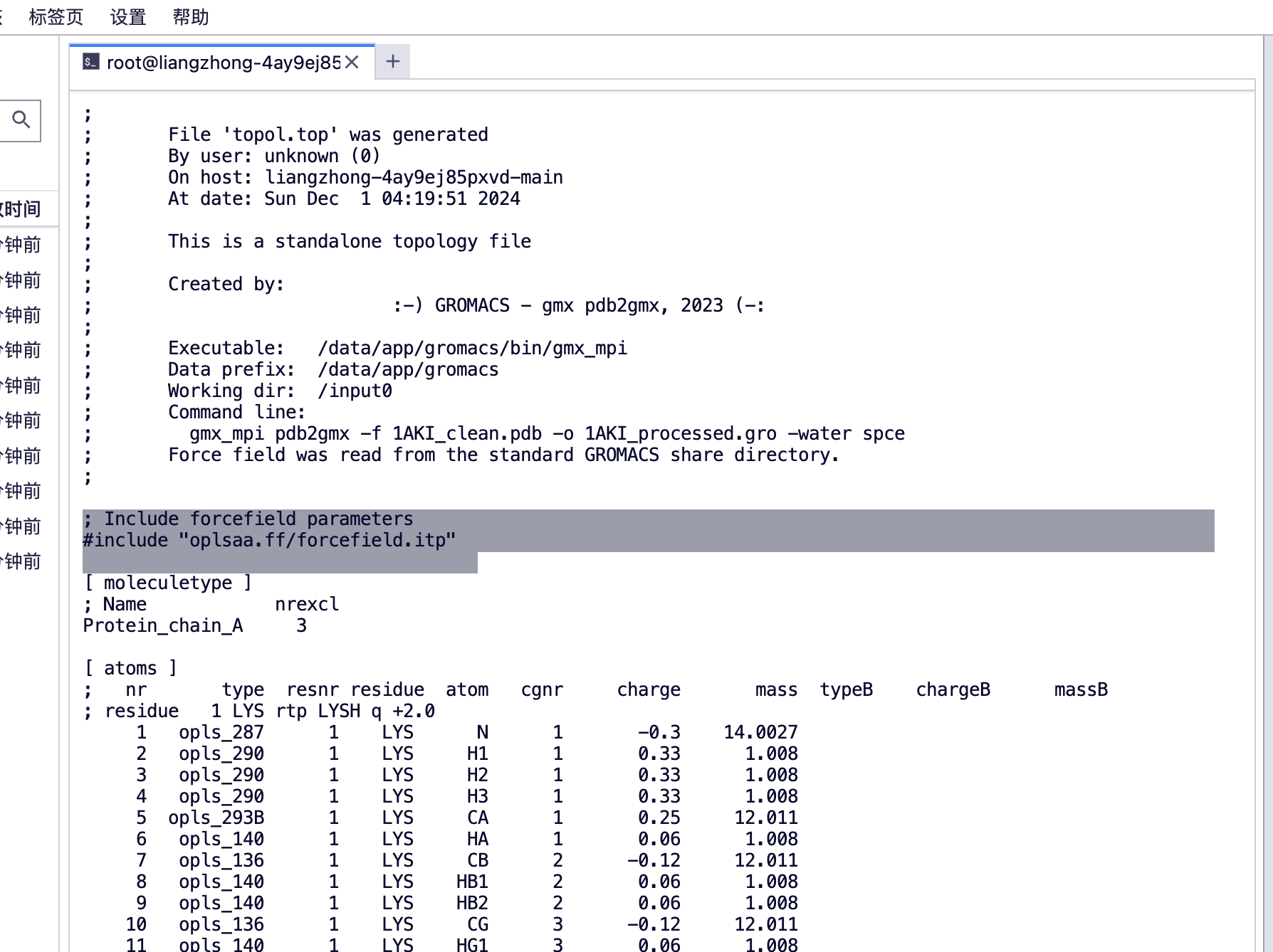
Use vim command to view topol.top and you can see the force field tag.
(base) root@liangzhong-4ay9ej85pxvd-main:/input0# ls
1AKI_clean.pdb      1aki.pdb  md.mdp     npt.mdp  posre.itp
1AKI_processed.gro  ions.mdp  minim.mdp  nvt.mdp  topol.top
4. Create a rhombic dodecahedron box to enclose the protein so that we can add solvent molecules
• Box shape selection: Common simulation box shapes include cube, orthogonal box, rhombic dodecahedron, etc. Shapes that can effectively fill molecules and reduce the amount of calculation are usually chosen.
gmx_mpi editconf -f 1AKI_processed.gro -o 1AKI_newbox.gro -c -d 1.0 -bt cubic

#将蛋白质在框中居中(-c),并将其放置在框边缘至少 1.0 nm 的位置(-d 1.0)

Command line:
  gmx_mpi editconf -f 1AKI_processed.gro -o 1AKI_newbox.gro -c -d 1.0 -bt cubic

Note that major changes are planned in future for editconf, to improve usability and utility.
Read 1960 atoms
Volume: 123.376 nm^3, corresponds to roughly 55500 electrons
No velocities found
    system size :  3.817  4.234  3.454 (nm)
    diameter    :  5.010               (nm)
    center      :  2.781  2.488  0.017 (nm)
    box vectors :  5.906  6.845  3.052 (nm)
    box angles  :  90.00  90.00  90.00 (degrees)
    box volume  : 123.38               (nm^3)
    shift       :  0.724  1.017  3.488 (nm)
new center      :  3.505  3.505  3.505 (nm)
new box vectors :  7.010  7.010  7.010 (nm)
new box angles  :  90.00  90.00  90.00 (degrees)
new box volume  : 344.48               (nm^3)
5. Define a box and add solvent (water)
Purpose:Solvation: Place molecules into a solvent environment (such as a water box) to simulate their behavior in the real environment.
gmx_mpi solvate -cp 1AKI_newbox.gro -cs spc216.gro -o 1AKI_solv.gro -p topol.top

#结果
Generating solvent configuration
Will generate new solvent configuration of 4x4x4 boxes
Solvent box contains 39252 atoms in 13084 residues
Removed 5451 solvent atoms due to solvent-solvent overlap
Removed 1869 solvent atoms due to solute-solvent overlap
Sorting configuration
Found 1 molecule type:
    SOL (   3 atoms): 10644 residues
Generated solvent containing 31932 atoms in 10644 residues
Writing generated configuration to 1AKI_solv.gro

Output configuration contains 33892 atoms in 10773 residues
Volume                 :     344.484 (nm^3)
Density                :     997.935 (g/l)
Number of solvent molecules:  10644

Processing topology
Adding line for 10644 solvent molecules with resname (SOL) to topology file (topol.top)

#查看一下 top 文件
(base) root@liangzhong-4ay9ej85pxvd-main:/input0# ls
'#topol.top.1#'   1AKI_newbox.gro      1AKI_solv.gro   ions.mdp   minim.mdp   nvt.mdp     topol.top
 1AKI_clean.pdb   1AKI_processed.gro   1aki.pdb        md.mdp     npt.mdp     posre.itp
(base) root@liangzhong-4ay9ej85pxvd-main:/input0# vim topol.top
#查看 top 文件的末尾
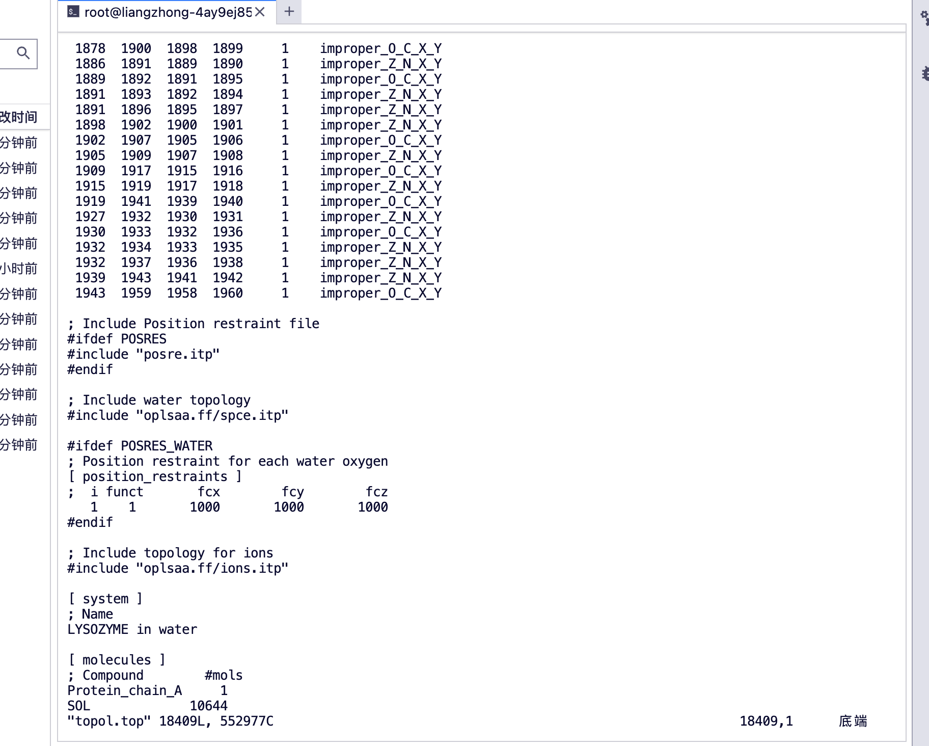
You can see [molecules]
protein_chain_A, protein A chain
SOL Water Molecule
6. Assemble the .tpr file
gmx_mpi grompp -f ions.mdp -c 1AKI_solv.gro -p topol.top -o ions.tpr
7. Neutralize the charge and replace the solvent molecules with ions
Charge Neutralization:Add ions (such as Na⁺, Cl⁻) to neutralize the total charge of the system and avoid simulation distortion caused by electrostatic effects.
gmx_mpi genion -s ions.tpr -o 1AKI_solv_ions.gro -p topol.top -pname NA -nname CL -neutral
Command line:
gmx_mpi genion -s ions.tpr -o 1AKI_solv_ions.gro -p topol.top -pname NA -nname CL -neutral
Reading file ions.tpr, VERSION 2023 (single precision)
Reading file ions.tpr, VERSION 2023 (single precision)
Will try to add 0 NA ions and 8 CL ions.
Select a continuous group of solvent molecules
Group 0 ( System) has 33892 elements
Group 1 ( Protein) has 1960 elements
Group 2 ( Protein-H) has 1001 elements
Group 3 ( C-alpha) has 129 elements
Group 4 ( Backbone) has 387 elements
Group 5 ( MainChain) has 517 elements
Group 6 ( MainChain+Cb) has 634 elements
Group 7 ( MainChain+H) has 646 elements
Group 8 ( SideChain) has 1314 elements
Group 9 ( SideChain-H) has 484 elements
Group 10 ( Prot-Masses) has 1960 elements
Group 11 ( non-Protein) has 31932 elements
Group 12 ( Water) has 31932 elements
Group 13 ( SOL) has 31932 elements
Group 14 ( non-Water) has 1960 elements
Select a group: 13
Selected 13: 'SOL'
Number of (3-atomic) solvent molecules: 10644
Processing topology
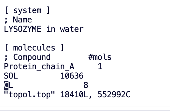
Replacing 8 solute molecules in topology file (topol.top) by 0 NA and 8 CL ions.
Back Off! I just backed up topol.top to ./#topol.top.2#
Using random seed -1212354563.
Replacing solvent molecule 3671 (atom 12973) with CL
Replacing solvent molecule 2264 (atom 8752) with CL
Replacing solvent molecule 2559 (atom 9637) with CL
Replacing solvent molecule 8081 (atom 26203) with CL
Replacing solvent molecule 8468 (atom 27364) with CL
Replacing solvent molecule 7439 (atom 24277) with CL
Replacing solvent molecule 9983 (atom 31909) with CL
Replacing solvent molecule 650 (atom 3910) with CL
GROMACS reminds you: "Water is just water" (Berk Hess)
(base) root@liangzhong-4ay9ej85pxvd-main:/input0#
It can be seen that a lot of chloride ions have been added
8. Energy Minimization
8.1 Reason: When we conduct molecular dynamics simulation, the pdb files we obtain are obtained through x-ray, electron microscopy and other methods, which contain many bond angles and distortions with excessive energy, or the formation or breaking of hydrogen bonds, special arrangements between molecules, and high energy caused by the close distance between atoms, making it difficult for the molecular system in the simulation to change from a high energy state to a low energy state. At this time, this method is needed to minimize the energy of the system.
8.2 Principle: The basic principle of energy minimization: Energy minimization is based on the potential energy function, which reduces the total potential energy of the system by iteratively calculating and adjusting the atomic coordinates. Commonly used methods include:
① Conjugate Gradient Method: A gradient descent method that accelerates convergence by utilizing information from the previous step.
② Steepest Descent Method: Each iteration moves in the opposite direction of the potential energy gradient, reducing energy along the steepest descent path.
③Newton-Raphson Method: A second-order derivative method that uses the second-order derivative of the potential energy function to more accurately find the minimum energy point.
8.3 Objective: To find a more stable molecular conformation by adjusting the atomic coordinates of the molecule to reduce the total potential energy of the system.
① Remove unreasonable geometric conformations: Through energy minimization, unreasonable geometric conformations in the initial structure, such as unreasonable atomic overlap and stretching, can be removed, the high energy state caused by them can be eliminated, and the system can be made more stable.
② Prepare the initial structure: Make sure the initial structure is in a low potential energy state to avoid unnecessary high energy impact during the simulation.
③ Improve computational efficiency: By reducing the total potential energy of the system, the stability and efficiency of subsequent simulations and calculations can be improved
gmx_mpi grompp -f minim.mdp -c 1AKI_solv_ions.gro -p topol.top -o em.tpr
gmx_mpi mdrun -v -deffnm em
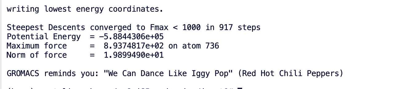
9. Take a look at the results (at the end of the tutorial, we will teach you how to visualize xvg files. You can use xmgrace, qtgrace, python, excel to make a graph. It is essentially a line graph)
gmx_mpi energy -f em.edr -o potential.xvg
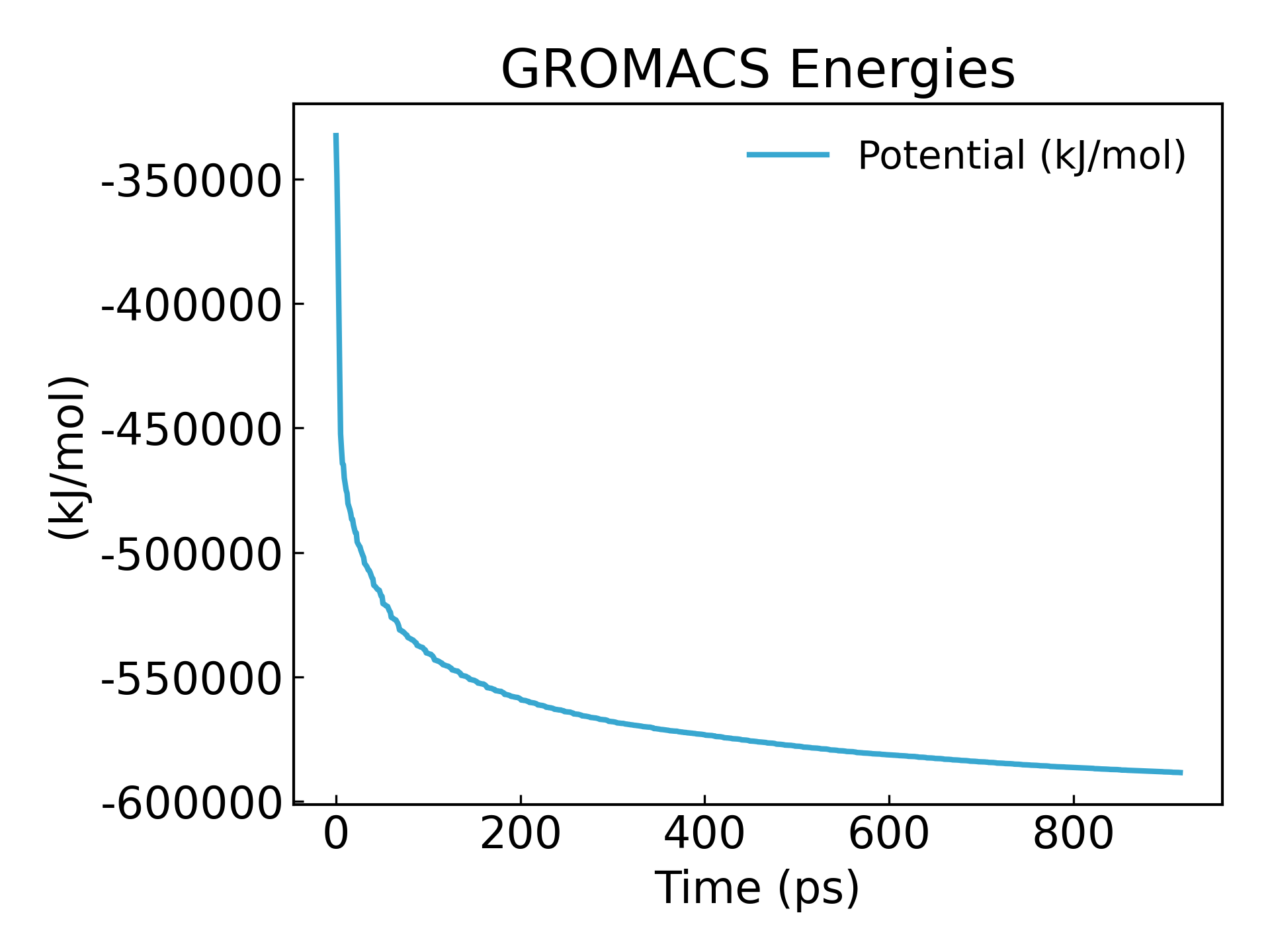
It can be seen that the energy is minimized to -600000 kj/mol
10. System balance
Objective: To adjust the system to the target temperature and pressure conditions to make it close to the real physical state.
(1) NVT simulation (constant volume and constant temperature):
• A constant volume and constant temperature ensemble is used to stabilize the temperature of the system to a target value.
• Temperature controller: Commonly used are Berendsen temperature coupler or V-rescale (modified weak coupling method), which controls the temperature by adjusting the atomic speed.
(2) NPT simulation (constant pressure and constant temperature):
• The constant pressure and constant temperature ensemble further adjusts the system density to a target value (usually the density of liquid water ~1 g/cm³).
• Pressure controller: Commonly used are Berendsen pressure coupler or Parrinello-Rahman pressure control method.
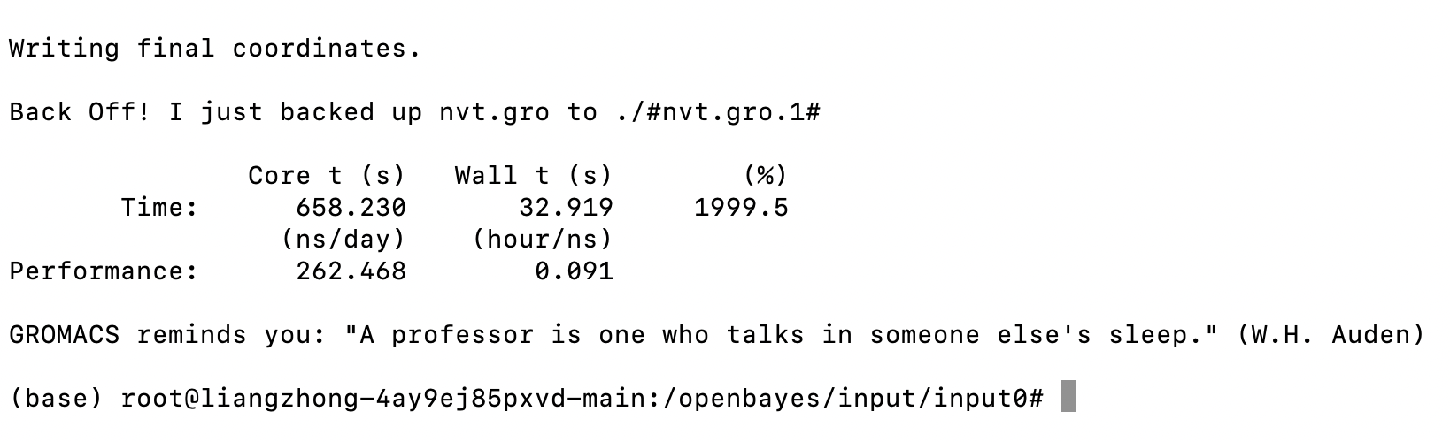
10.1. Perform NVT equilibration for 100 ps, which is performed under (constant particle number, volume and temperature), also known as "isothermal and isochoric"
It is very fast with GPU acceleration, taking only 10+ seconds.
gmx_mpi grompp -f nvt.mdp -c em.gro -r em.gro -p topol.top -o nvt.tpr

gmx_mpi mdrun -deffnm nvt -nb gpu -pme cpu
#将 PME 任务移至 CPU
gmx_mpi energy -f nvt.edr -o temperature.xvg
#生成温度随时间变化的图像,查看温度是否平衡
16
0
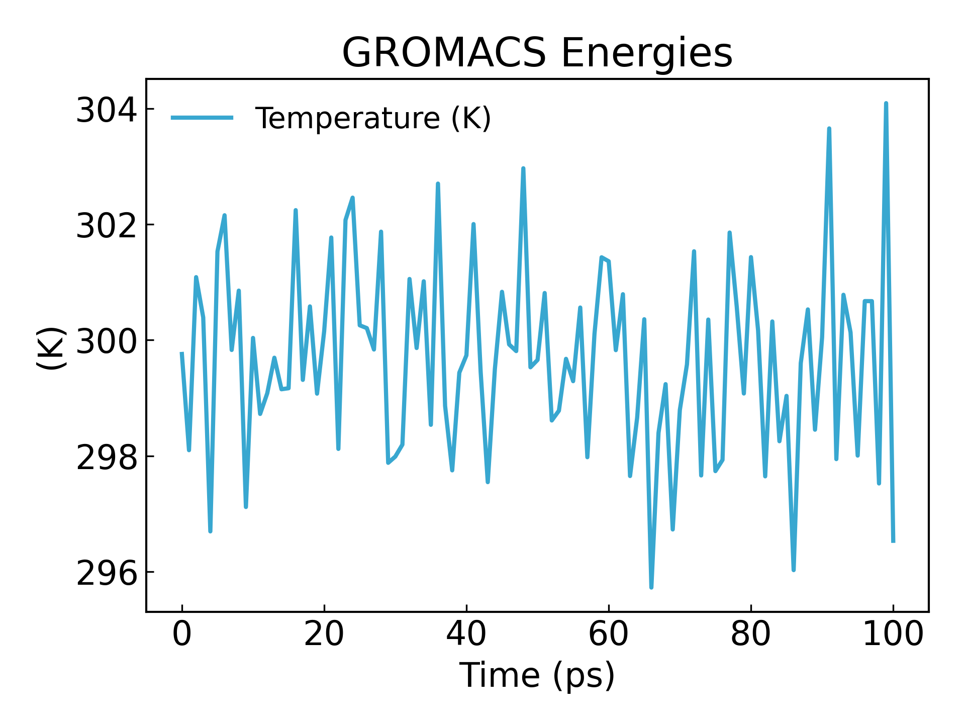
It can be seen that the temperature also reaches a basic steady state within 100ps
10.2. NPT “isothermal and isobaric” balance, stabilize the system pressure, and perform 100 ps NPT balance.
gmx_mpi grompp -f npt.mdp -c nvt.gro -r nvt.gro -t nvt.cpt -p topol.top -o npt.tpr
gmx_mpi mdrun -deffnm npt -nb gpu -pme cpu
#压力是否平衡
gmx_mpi energy -f npt.edr -o pressure.xvg
18
0
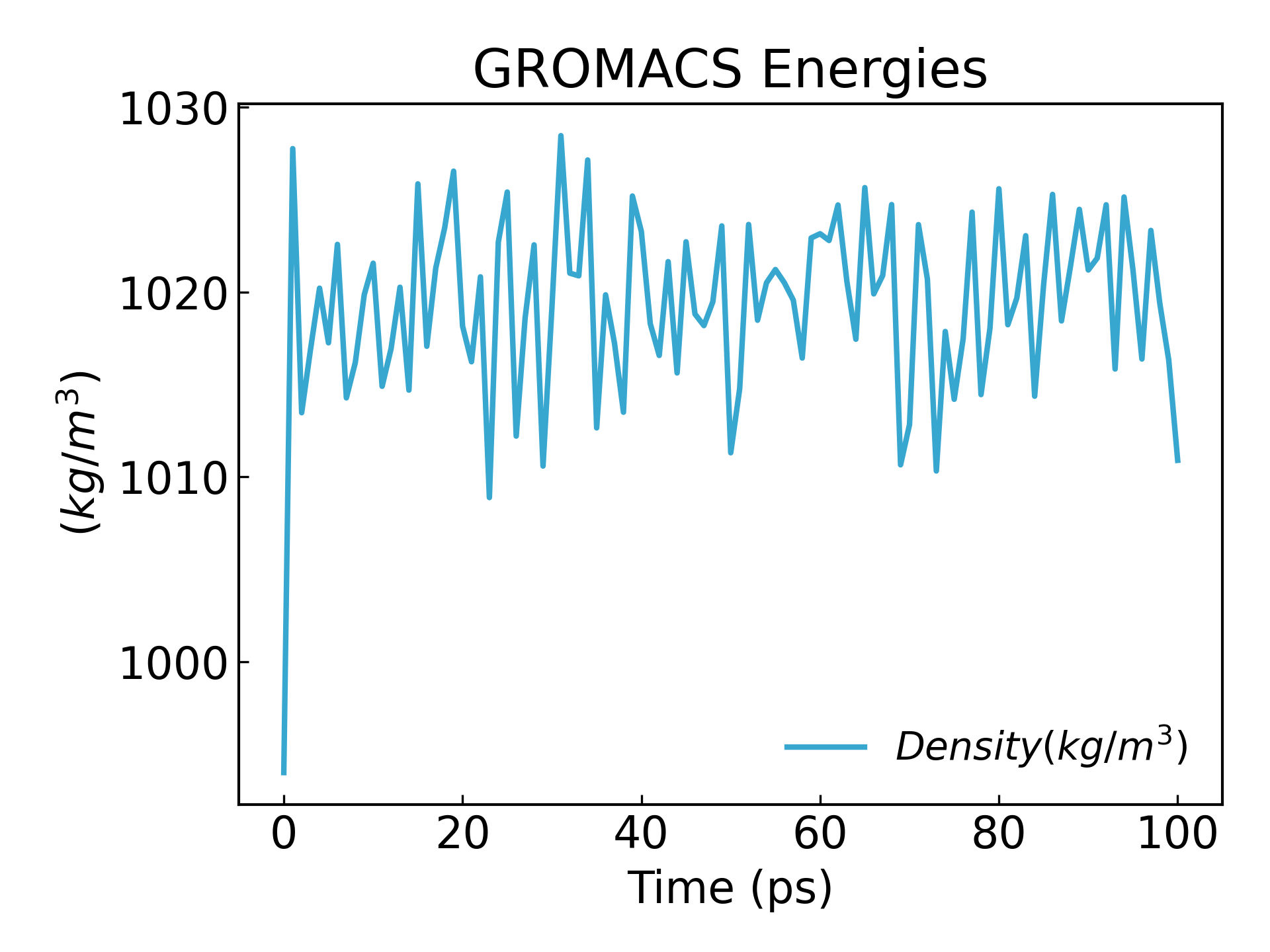
gmx_mpi energy -f npt.edr -o density.xvg
24
0
We can see that the density reaches a steady state:
11. After completing the 2 equilibration phases, the system is now well equilibrated at the desired temperature and pressure. We can now release the positional constraints and run MD.
You can modify the time according to your needs. This tutorial simulates 100ns.
Time step dt = 2 fs (common setting):
50000000 steps, with a time step of 2 fs, equivalent to 100 nanoseconds (ns)
50000000 x2 fs = 10^8 fs = 10^5 ps =100ns
vim md.mdp
nsteps                  = 50000000    ; 2 * 50000000 = 100000 ps (100 ns)
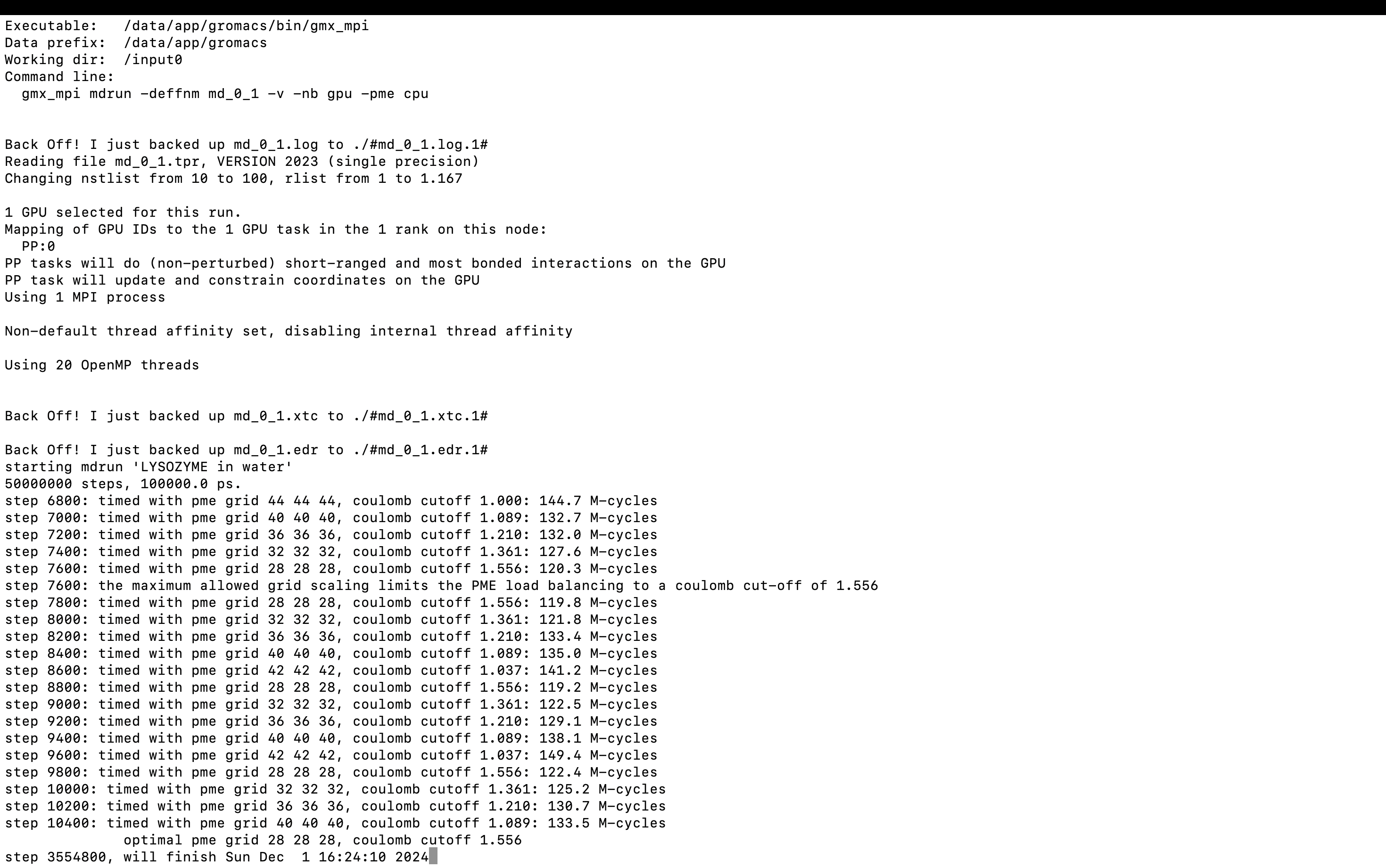
gmx_mpi grompp -f md.mdp -c npt.gro -t npt.cpt -p topol.top -o md_0_1.tpr

##最后一步提交,pme 分配到 CPU 上:
gmx_mpi mdrun -deffnm md_0_1 -v -nb gpu -pme cpu
-v can display the remaining time of the run.
3. Results Analysis
1. trjconv, which is used as a post-processing tool to remove coordinates, correct periodicity or manually modify trajectories (time units, frame rates, etc.). This is because in all simulations with periodic boundary conditions, molecules may break or jump around the edges of the box. It can re-center the molecule in the box, rewrap the molecule, and restore the rhombic dodecahedral shape of the box.
-pbc mol: 去除轨迹中的周期性边界条件 (PBC),并基于分子进行修正(即确保每个分子在轨迹中是完整的)。
•	-center: 将选定的分子/分组居中到模拟框的中心。
gmx_mpi trjconv -s md_0_1.tpr -f md_0_1.xtc -o md_0_1_noPBC.xtc -pbc mol -center

Select group for centering
Group     0 (         System) has 33876 elements
Group     1 (        Protein) has  1960 elements
Group     2 (      Protein-H) has  1001 elements
Group     3 (        C-alpha) has   129 elements
Group     4 (       Backbone) has   387 elements
Group     5 (      MainChain) has   517 elements
Group     6 (   MainChain+Cb) has   634 elements
Group     7 (    MainChain+H) has   646 elements
Group     8 (      SideChain) has  1314 elements
Group     9 (    SideChain-H) has   484 elements
Group    10 (    Prot-Masses) has  1960 elements
Group    11 (    non-Protein) has 31916 elements
Group    12 (          Water) has 31908 elements
Group    13 (            SOL) has 31908 elements
Group    14 (      non-Water) has  1968 elements
Group    15 (            Ion) has     8 elements
Group    16 ( Water_and_ions) has 31916 elements
Select a group: 1
Selected 1: 'Protein'
Select group for output
Group     0 (         System) has 33876 elements
Group     1 (        Protein) has  1960 elements
Group     2 (      Protein-H) has  1001 elements
Group     3 (        C-alpha) has   129 elements
Group     4 (       Backbone) has   387 elements
Group     5 (      MainChain) has   517 elements
Group     6 (   MainChain+Cb) has   634 elements
Group     7 (    MainChain+H) has   646 elements
Group     8 (      SideChain) has  1314 elements
Group     9 (    SideChain-H) has   484 elements
Group    10 (    Prot-Masses) has  1960 elements
Group    11 (    non-Protein) has 31916 elements
Group    12 (          Water) has 31908 elements
Group    13 (            SOL) has 31908 elements
Group    14 (      non-Water) has  1968 elements
Group    15 (            Ion) has     8 elements
Group    16 ( Water_and_ions) has 31916 elements
Select a group: 0
Selected 0: 'System'
Selection 4 (“Backbone”) was used for least squares fitting and RMSD calculations.
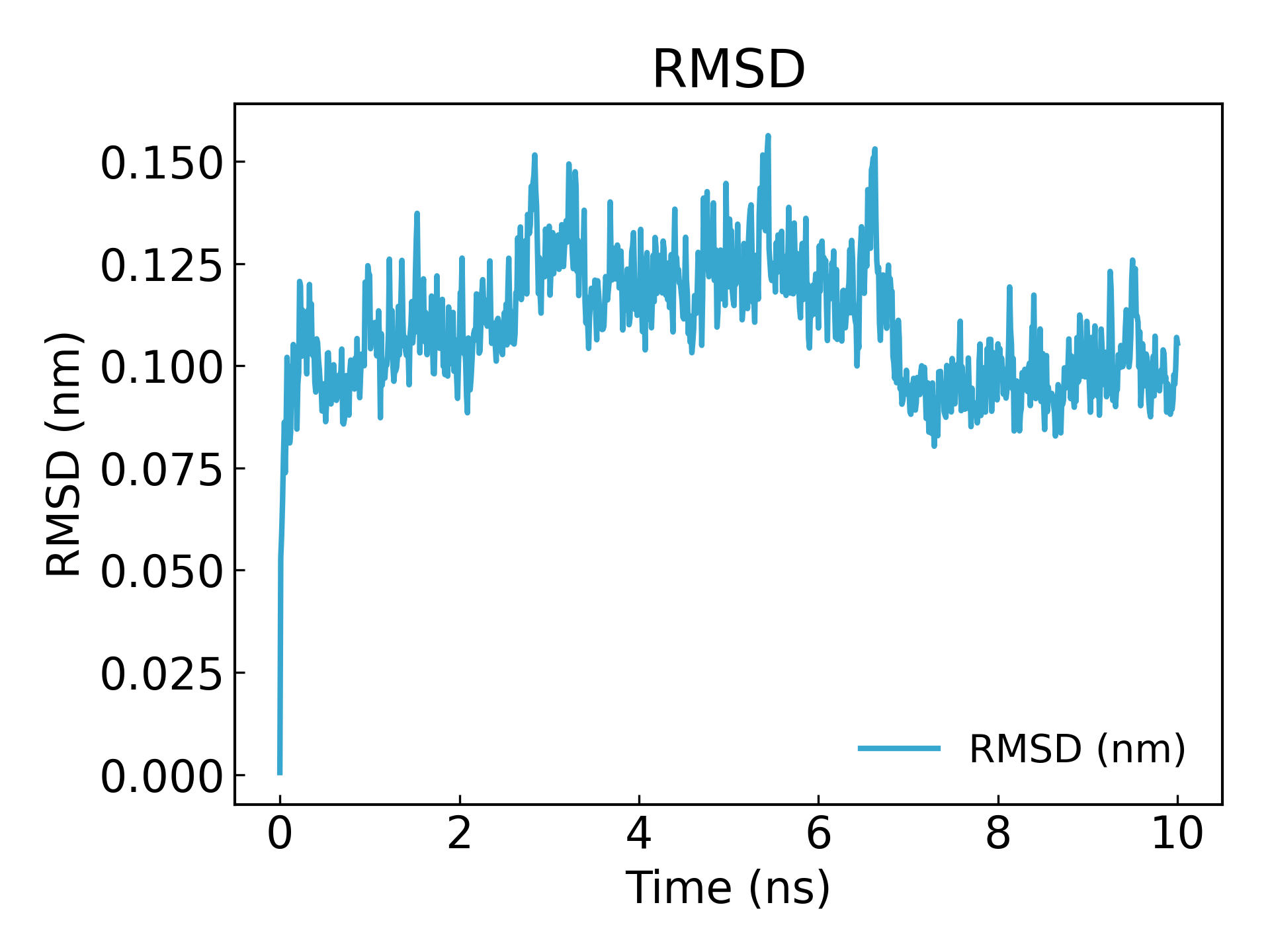
2.RMSD
Can be used to check the convergence of the simulation and the stability of the protein.g_rms**The RMSD of the structure during the simulation and the initial structure, the deviation of the structure at a certain moment relative to 0ns, is often used to evaluate the stability of protein structure. It is often used in the field of drug design, such as the stability of protein ligand structure. The fluctuation range of the RMSD curve is small and stable, indicating that the affinity between the ligand and the receptor is large.
gmx_mpi rms -s md_0_1.tpr -f md_0_1_noPBC.xtc -o rmsd.xvg
Select 4 ("Backbone") for least squares fitting and RMSD calculation
It can be seen that equilibrium is reached after 10ns (Note: When publishing or submitting an article, it is best to simulate for 100ns or 50ns)
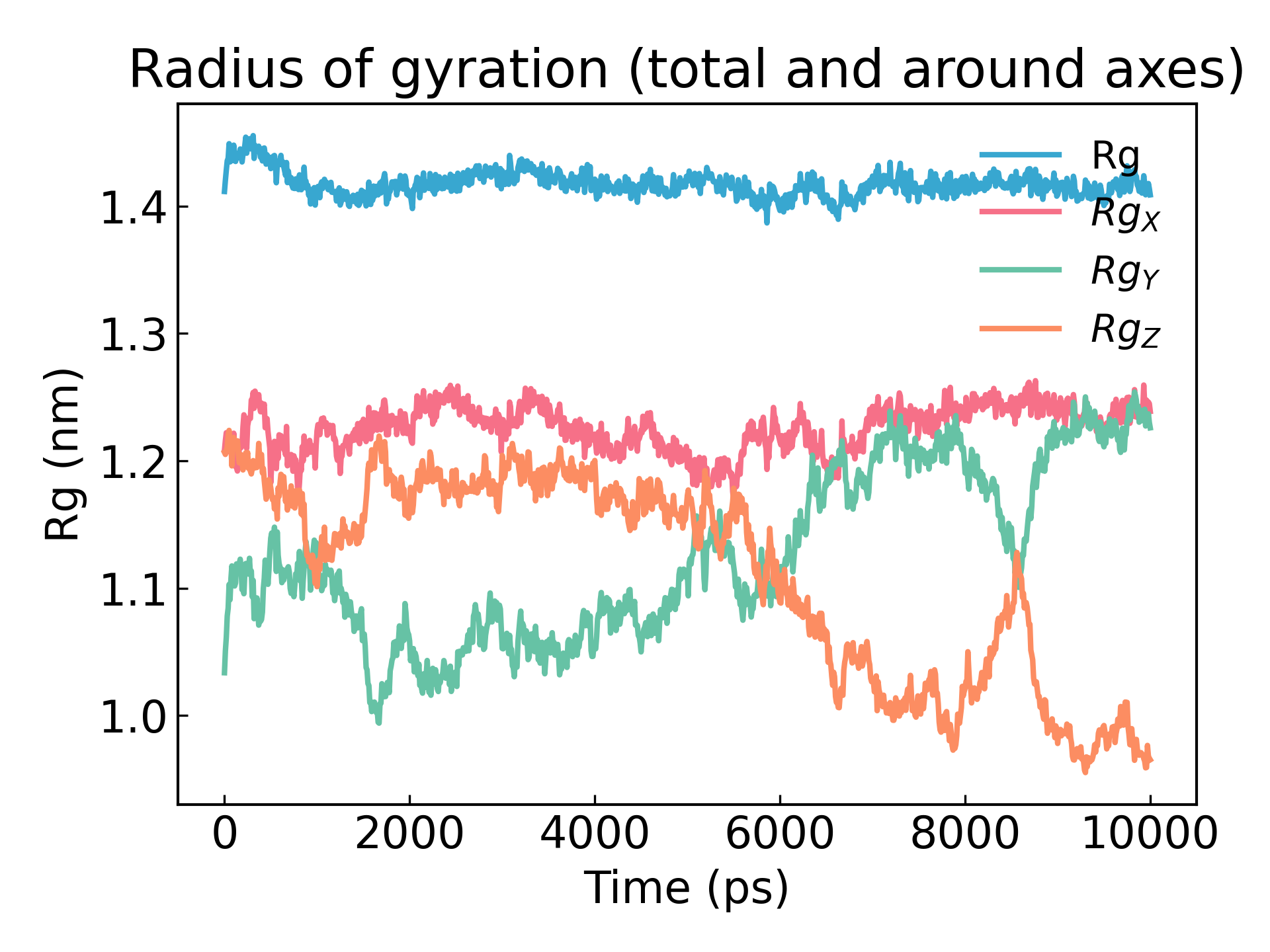
3. Gyration radius analysis
gmx_mpi gyrate -s md_0_1.tpr -f md_0_1_noPBC.xtc -o gyrate.xvg
The radius of gyration of a protein is a measure of its compactness. If a protein structure is stable, it will likely maintain a relatively constant R g value. If a protein unfolds, its R g value will change over time. Let's analyze the radius of gyration of lysozyme in our simulation:
4. Visualization
Recommended Software:DuIvyTools: GROMACS simulation analysis and visualization tools
From:https://github.com/CharlesHahn/DuIvyTools
pip install DuIvyTools

dit xvg_show -f rmsd.xvg -o rmsd_plot.png

dit xvg_show -f rmsd.xvg -o rmsd_plot.png

dit xvg_show -f potential.xvg -o potential_plot.png

dit xvg_show -f temperature.xvg -o temperature_plot.png

dit xvg_show -f density.xvg -o density_plot.png
dit xvg_show -f pressure.xvg -o pressure_plot.png
Open the dataset we created
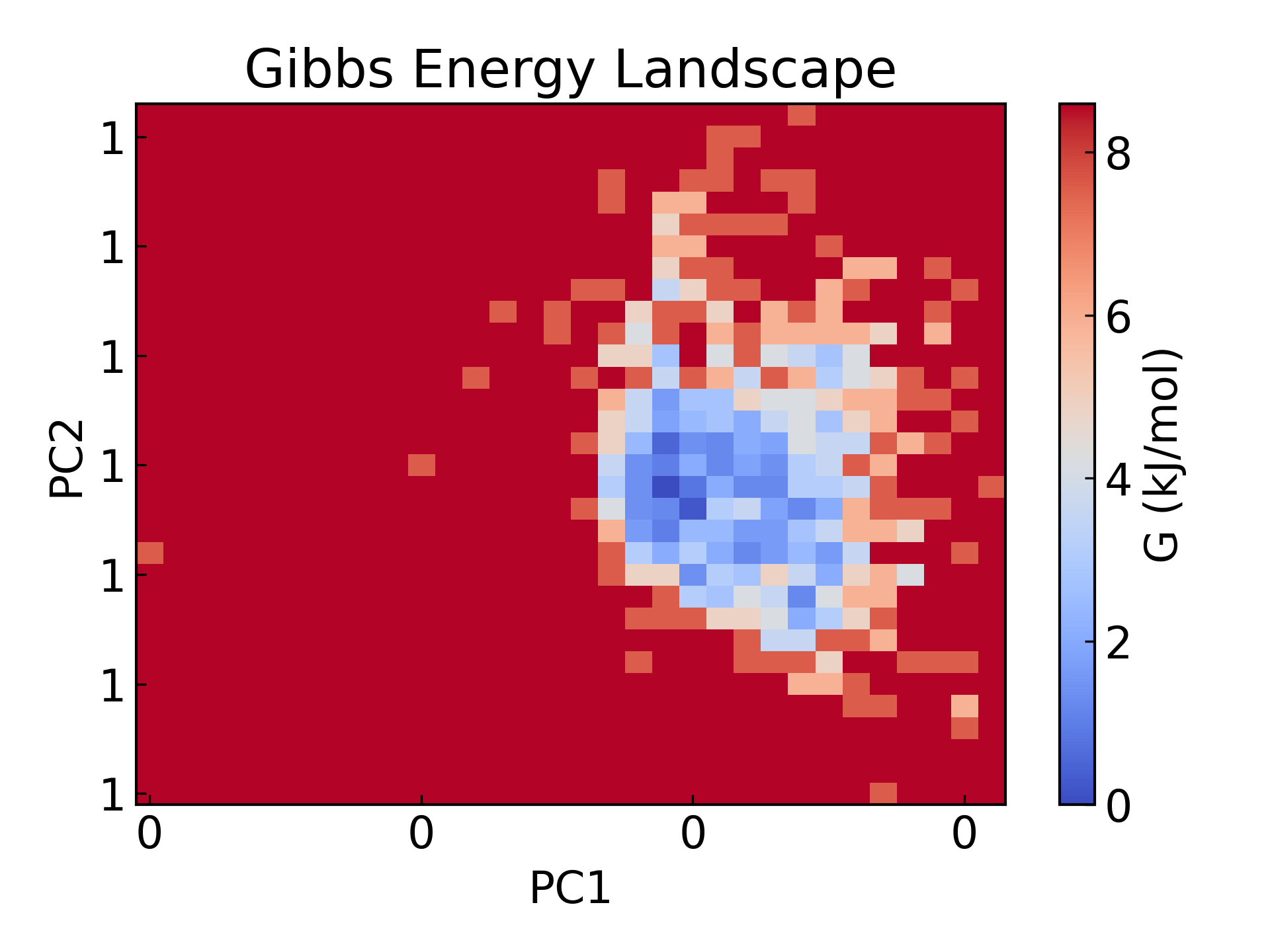
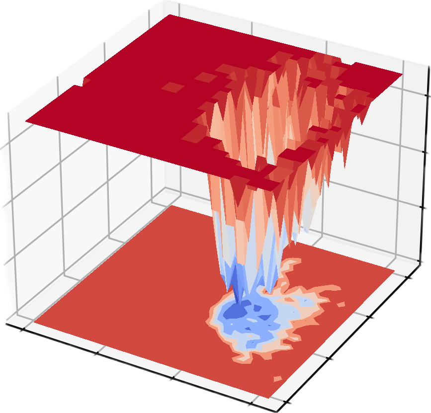
5. GROMACS energy landscape mapping The free energy landscape was plotted, with the gyration radius and rmsd as two PCA components respectively.
gmx_mpi gyrate -s md_0_1.tpr -f md_0_1_noPBC.xtc -o rg.xvg
gmx_mpi rms -s md_0_1.tpr -f md_0_1_noPBC.xtc -o rmsd.xvg
vim rmsd.xvg
#输入以下命令删除以 # 或 @ 开头的行:
:g/^[@#]/d

vim rg.xvg
#输入以下命令删除以 # 或 @ 开头的行:
:g/^[@#]/d

#注意不要有空行,
paste rmsd.xvg rg.xvg > rmsd-rg.xvg

(base) # tail -f rmsd-rg.xvg
9910.0000000    0.0925907	      9910     1.37624     1.20925     1.20765    0.931324
9920.0000000    0.0881348	      9920     1.38369     1.22248     1.21078    0.932077
9930.0000000    0.0911074	      9930     1.39224     1.23799     1.21709    0.928842
9940.0000000    0.0893596	      9940     1.38188     1.21942     1.21672    0.922916
9950.0000000    0.0915931	      9950     1.37509     1.21939     1.20194    0.922051
9960.0000000    0.0978161	      9960     1.38113      1.2262     1.21084    0.919414
9970.0000000    0.0954911	      9970     1.37934     1.21241     1.20711    0.937075
9980.0000000    0.0993617	      9980     1.38301     1.22353     1.21083     0.92862
9990.0000000    0.1069279	      9990     1.37943     1.22317     1.20579    0.924978
10000.0000000    0.1055321	     10000     1.37524     1.21648     1.20194     0.92632
^Z
[11]+  Stopped                 tail -f rmsd-rg.xvg
#查看已经将两个文件整合在一起了,我们只要保留
#从 rmsd-rg.xvg 文件内容可以看到,每一行的数据格式如下:
时间_RMSD(ns)    RMSD	      时间_Rg(ps)     Rg 其他列

(base) tail -f rmsd.xvg
9910.0000000    0.0925907
9920.0000000    0.0881348
9930.0000000    0.0911074
9940.0000000    0.0893596
9950.0000000    0.0915931
9960.0000000    0.0978161
9970.0000000    0.0954911
9980.0000000    0.0993617
9990.0000000    0.1069279
10000.0000000    0.1055321
^Z
[12]+  Stopped                 tail -f rmsd.xvg

#整理数据为
时间 (ns)    RMSD    Rg

(base) python
Python 3.8.15 (default, Nov 24 2022, 15:19:38)
[GCC 11.2.0] :: Anaconda, Inc. on linux
Type "help", "copyright", "credits" or "license" for more information.
# 加载数据
>>> import pandas as pd
>>> data = pd.read_csv("rmsd-rg.xvg", delim_whitespace=True, header=None, comment="#")
# 保留需要的列:第 1 列 (RMSD 时间) 、第 2 列 (RMSD) 、第 4 列 (Rg)
>>> cleaned_data = data[[0, 1, 3]]
# 将列名修改为更直观的名称
>>> cleaned_data.columns = ["Time (ps)", "RMSD", "Rg"]
>>> cleaned_data.to_csv("rmsd-rg-cleaned.xvg", sep="\t", index=False, header=False)
>>> exit()

#整理成功
tail -f rmsd-rg-cleaned.xvg
9910.0	0.0925907	1.37624
9920.0	0.0881348	1.38369
9930.0	0.0911074	1.39224
9940.0	0.0893596	1.38188
9950.0	0.0915931	1.37509
9960.0	0.0978161	1.38113
9970.0	0.0954911	1.37934
9980.0	0.0993617	1.38301
9990.0	0.1069279	1.37943
10000.0	0.1055321	1.37524

gmx_mpi sham -tsham 300 -nlevels 100 -f rmsd-rg-cleaned.xvg -ls gibbs.xpm -g gibbs.log -lsh enthalpy.xpm -lss entropy.xpm

dit xpm_show -f gibbs.xpm  -o gibbs_2d.png
dit xpm_show -f gibbs.xpm -m 3d -o gibbs_3d.png
#tsham : 设定温度
#-nlevels: 设定 FEL 的层次数量
Free Energy Landscape (FES) is a very important tool in molecular simulation, mainly used to describe the free energy distribution of a molecular system at a specific coordinate. Its core function is to reveal the thermodynamic stability and kinetic process of the system, and is usually of great significance in the following scientific research fields:
- Steady-state and transition-state studies: Reveal the stable conformation (free energy minimum point) and conformational conversion path (free energy barrier) of the system, which is used to analyze protein folding, chemical reactions and molecular recognition processes.
- Kinetic pathways and thermodynamic stability: Quantifying the free energy difference between different states helps understand the energy driving force of molecular interactions and conformational transitions.
- Drug design and catalysis research:Predict ligand-receptor binding pathways, energy barriers, and reaction rates, providing theoretical guidance for molecular mechanism analysis and functional optimization.
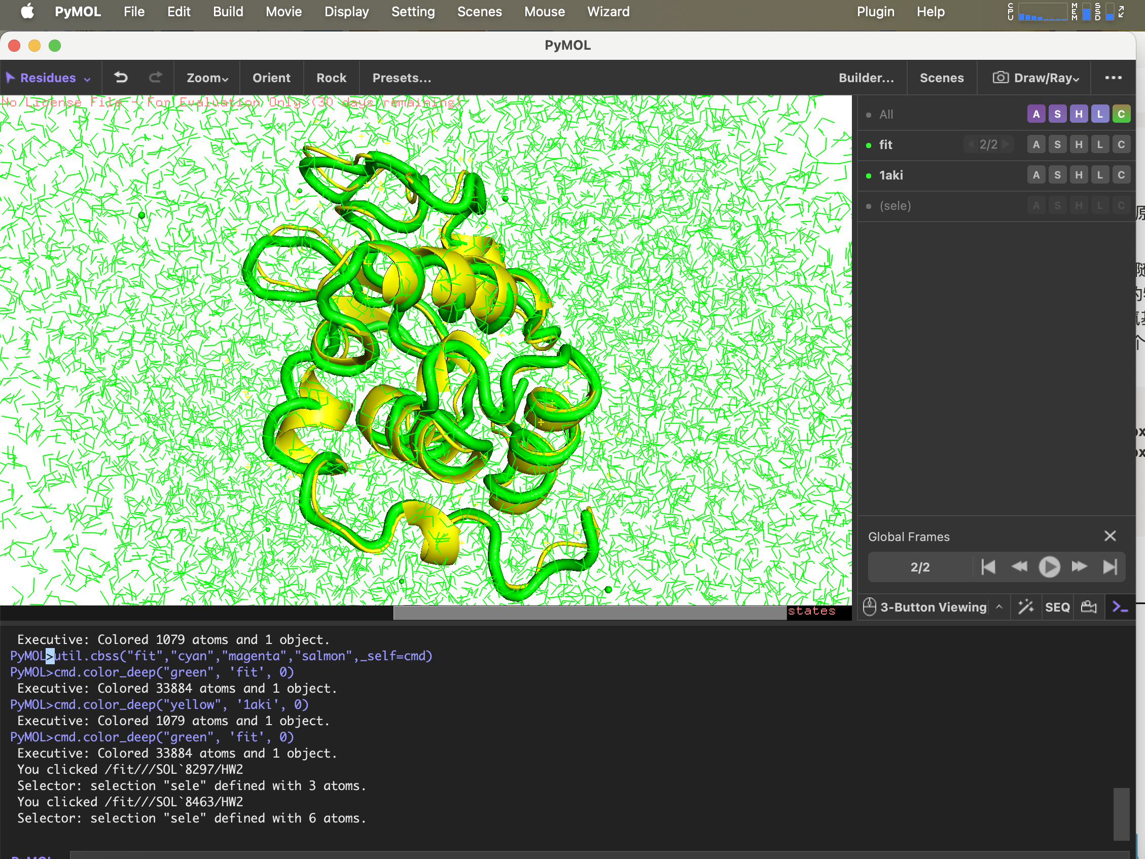
6.g_confrms Comparison of conformational differences
To compare the structure after simulation with the structure in the original PDB file,fit.pdb A file containing two molecular structures, select both 4 (Backbone)
gmx_mpi confrms -f1 1AKI_clean.pdb -f2 md_0_1.gro -o fit.pdb
pdb structure opened with pymol
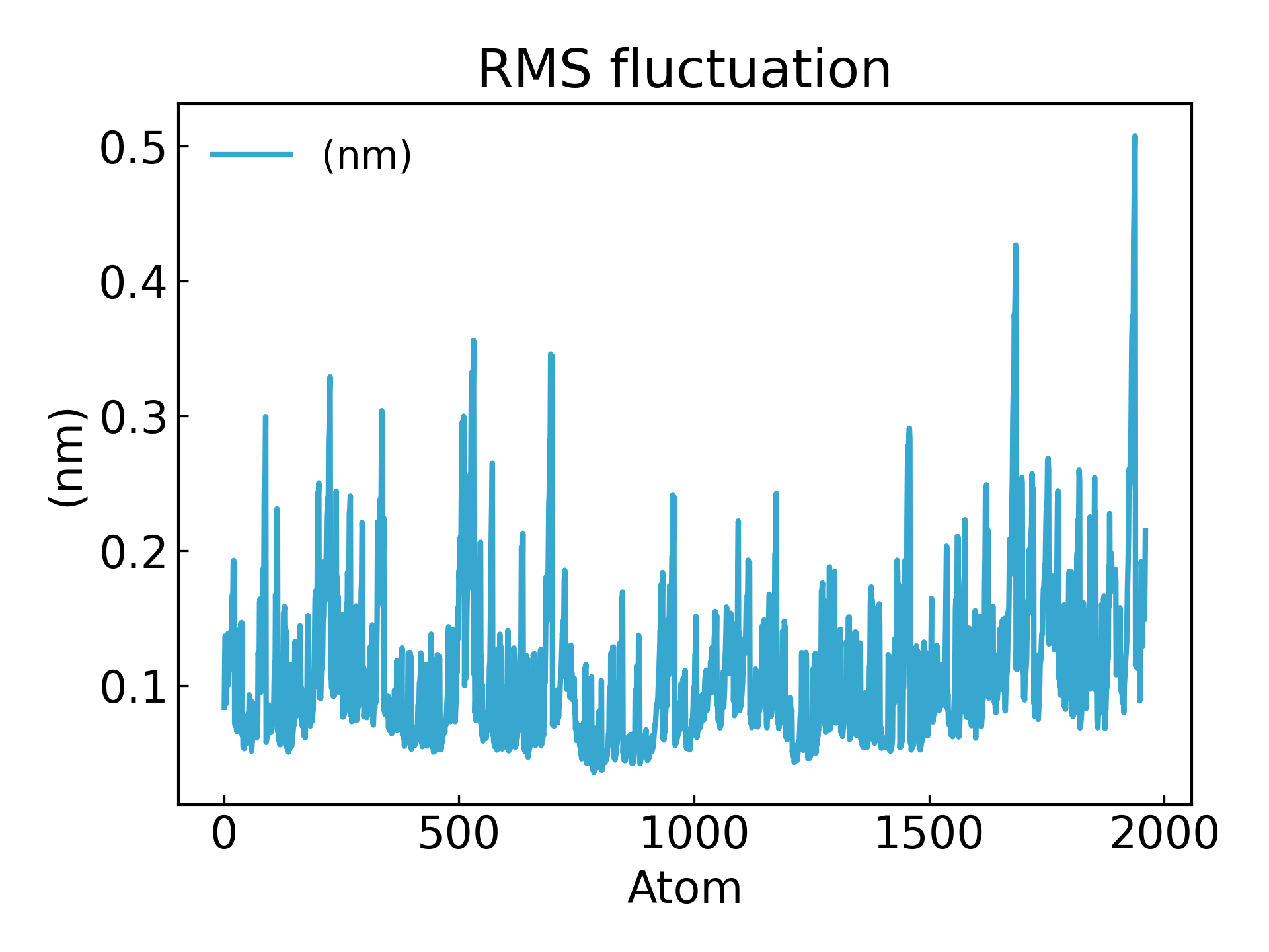
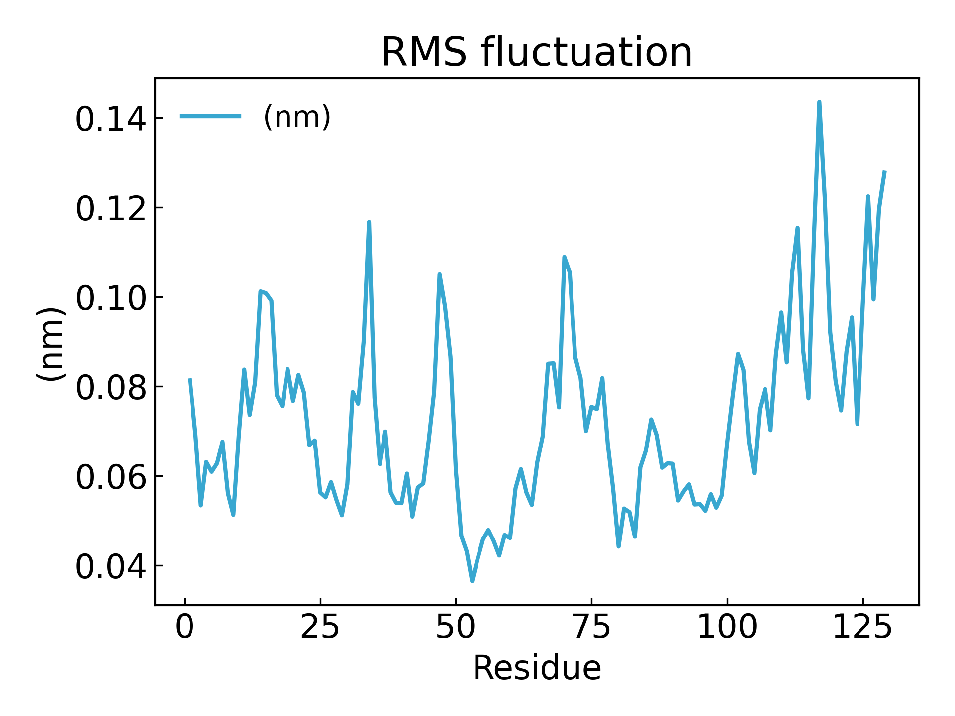
7.g_rmsf Calculate the root mean square fluctuation (RMSF) and the average structure within 500 ps after calculation.g_rmsf The result is a curve that changes with the atomic number. Select 1 Protein
The fluctuations of amino acid residues can be inferred using the RMSF parameter, which explains the average deviation of each amino acid residue/atom from a reference position over time. More precisely, it can be said to analyze the specific part of the protein structure that fluctuates from its average structure. Amino acids or amino acid groups with high RMSF values indicate that the complex has greater flexibility, while amino acids with low RMSF values indicate that the complex is less flexible. Frequent fluctuations are associated with poor stability. The RMSF value is a dynamic parameter that measures the average backbone flexibility at each residue position [19].
gmx_mpi rmsf -s md_0_1.tpr -f md_0_1_noPBC.xtc -b 500 -o fws-rmsf.xvg -ox fws-avg.pdb
gmx_mpi rmsf -s md_0_1.tpr -f md_0_1_noPBC.xtc -b 500 -o fws-rmsf.xvg -ox fws-avg.pdb -res

dit xvg_show -f fws-rmsf.xvg -o rmsf_res.png
# 最后可以放到 pymol 里面看轨迹动画,点击播放即可
gmx_mpi trjconv -s md_0_1.tpr -f md_0_1_noPBC.xtc -o trajectory.pdb -skip 10
Reference
Build AI with AI
From idea to launch — accelerate your AI development with free AI co-coding, out-of-the-box environment and best price of GPUs.