HyperAI超神经

In the second episode of the "Meet AI4S" series, we have the honor of inviting Li Yuzhe, a postdoctoral fellow in Zhang Qiangfeng's laboratory at the School of Life Sciences at Tsinghua University,His laboratory, Qiangfeng Zhang, belongs to the School of Life Sciences at Tsinghua University and is also an important part of the Tsinghua-Peking University Joint Center for Life Sciences and the Beijing Advanced Innovation Center for Structural Biology. The laboratory's research focuses on the intersection of life sciences and artificial intelligence algorithms, RNA structural group technology and algorithm development, single-cell genome sequencing technology and algorithm development, protein structure modeling based on cryo-electron microscopy data, and the development of related artificial intelligence algorithms.

This sharing,Dr. Li Yuzhe gave a speech titled "Exploring AI Applications in Genomics: Taking the Spatial Transcriptome Data Characterization Algorithm SPACE as an Example".The team’s latest research results were shared, and AI methods in spatial transcriptomics and single-cell omics research were introduced.

HyperAI has compiled and summarized Dr. Li Yuzhe's in-depth sharing without violating the original intention.

Click to view the full live replay:

AI for Science brings huge changes to the research paradigm in the scientific field

Today, the topic I will share is AI for Science. I believe that AI for Science has brought about major changes to the research paradigm in the entire scientific field. Next, I will explain it in detail using the research on protein structure as an example.

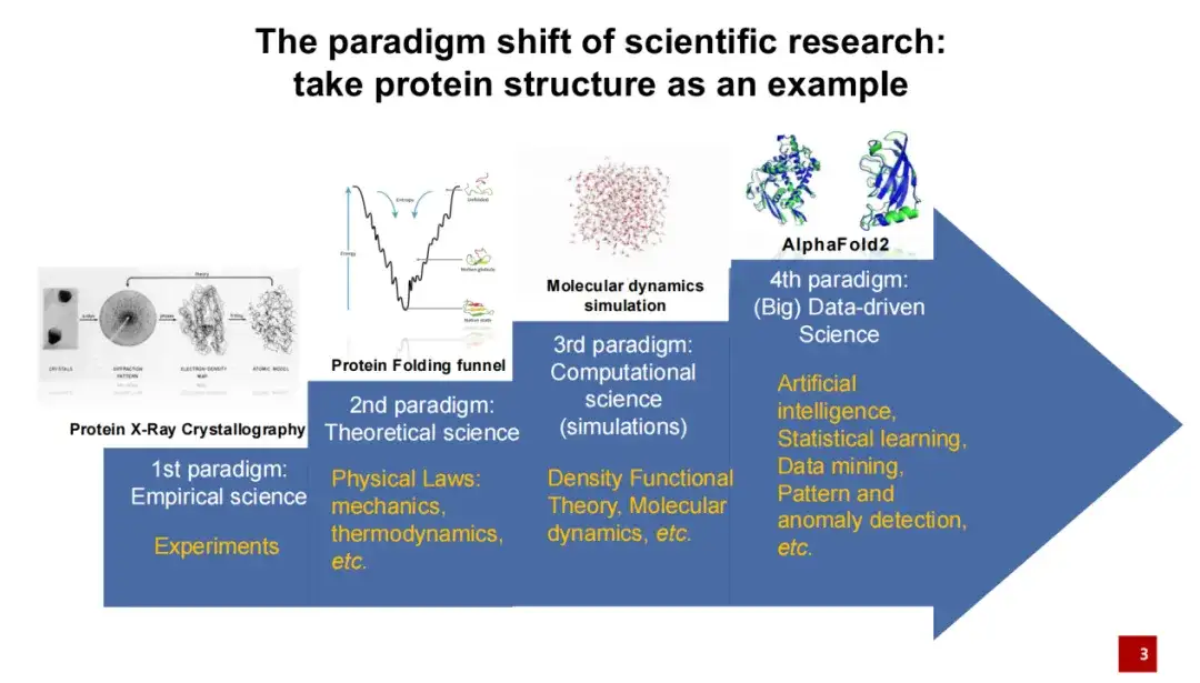
The first generation of protein structure research paradigm was mainly conducted through experimental means.That is, use X-rays to photograph the crystals formed by the protein, and then perform structural modeling.

The second generation of protein structure research paradigm was mainly led by physicists who added theoretical knowledge to the study of protein structure.For example, if the energy of a protein folding is low, then this folding is relatively stable.

The third generation of protein structure research paradigm refers to the 1990s, when, with the development of computer technology, computer simulation was gradually applied to protein structure research.In particular, molecular dynamics simulations have been widely used in recent years. These simulation methods help us to better calculate and predict protein structures to a certain extent. In recent years, especially in 2020, after artificial intelligence algorithms entered the field of protein structure, they brought another breakthrough. In the 2020 protein structure prediction competition, AlphaFold 2 was far ahead of other competition methods.

The introduction of artificial intelligence has brought about a huge paradigm shift in life sciences and the entire scientific research field. Compared with traditional research methods,Artificial intelligence places more emphasis on starting from data and conducting data-driven scientific research.This means that we no longer need to propose a scientific hypothesis in advance, but can learn and reveal the laws of nature directly from the data.

The evolution of AI for Genomics

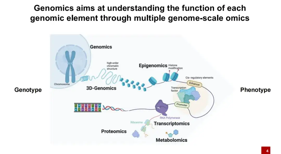
The following sharing will focus on the application of AI in the field of genomics. In short,Genomic research mainly explores the relationship between genotype (all the DNA in the body) and phenotype (individual characteristics such as height and weight).

As we all know, DNA is not naked in cells, but wrapped around nucleosomes. Nucleosomes are attached with many histone modifications. Normally, these DNAs are tightly wrapped together. Only under certain conditions will the DNA be exposed to form open intervals. At this time, proteins such as transcription factors can bind to these exposed DNA intervals.

In the subsequent transcription process, RNA can be transcribed by RNA polymerase, and then translated into protein by ribosome, and the protein finally plays a role in life activities.The research goal of genomics is to understand how various DNA elements affect life activities.

We summarize the important events and developments in the development of AI for Science since the DNA double helix structure was cracked in the 1950s to the recent development. Its beginning can be traced back to the discovery of the DNA double helix structure in the 1950s and the development of Sanger sequencing technology in the 1970s.

As shown in the figure below, the blue part represents the development of various sequencing technologies and experimental technologies; the green part represents important methods in the field of artificial intelligence; the yellow part represents the establishment of some important large-scale research plans and databases; the red part represents representative methods and applications in the field of AI for Genomics.

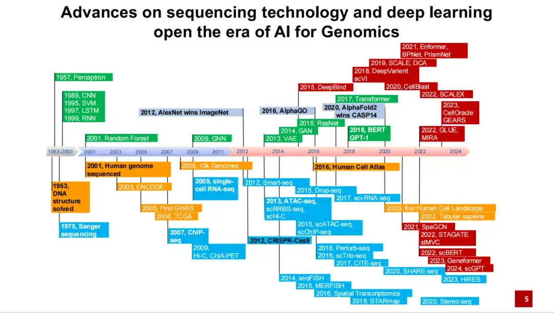
As you can see,2001, the draft of the Human Genome Project was initially completed, sequencing the entire DNA sequence of a white male. In 2012,AlexNet surpassed humans in image classification tasks for the first time, ushering in the explosive development of artificial intelligence over the past decade. In 2016,The Human Cell Atlas Project was proposed, and research gradually shifted from the DNA sequence of a single individual to all cells. In the same year, AlphaGo, based on the reinforcement learning method, defeated humans in the Go game.

For AI for Genomics or AI for Science,An important breakthrough was that in 2020, AlphaFold 2 took a far-leading first place in CASP 14.This has led to an increasing number of artificial intelligence methods being applied to the field of genomics.

in,Single-cell genomics is a major breakthrough in the field of genomics in recent years.Traditional genomic research usually involves bulk sequencing. Assume that each line in the figure below represents a cell, and lines of different colors represent different cell types. In the past, sequencing was done by mixing the entire tissue, making it difficult to determine which specific cell each DNA or RNA came from. The emergence of single-cell technology allows us to not only obtain all the DNA or RNA in the tissue, but also to identify the specific cell sources of these DNA or RNA. Because different cell types have different gene expressions and perform different functions, we can further understand life activities.

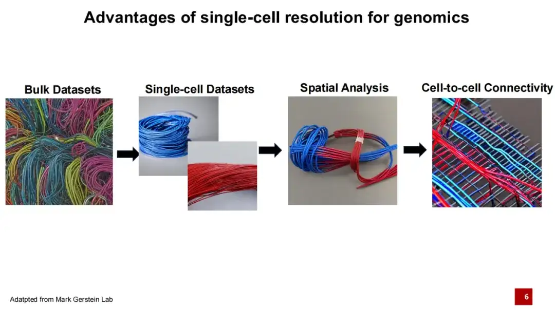
In the past five years, spatial omics technology represented by spatial transcriptomics has gone a step further based on single-cell omics technology.Not only can we obtain information about each cell type, but we can also determine the distribution of these cells in space.Because interactions between cells are an important basis for the realization of their functions, further research focuses on how cells are connected.

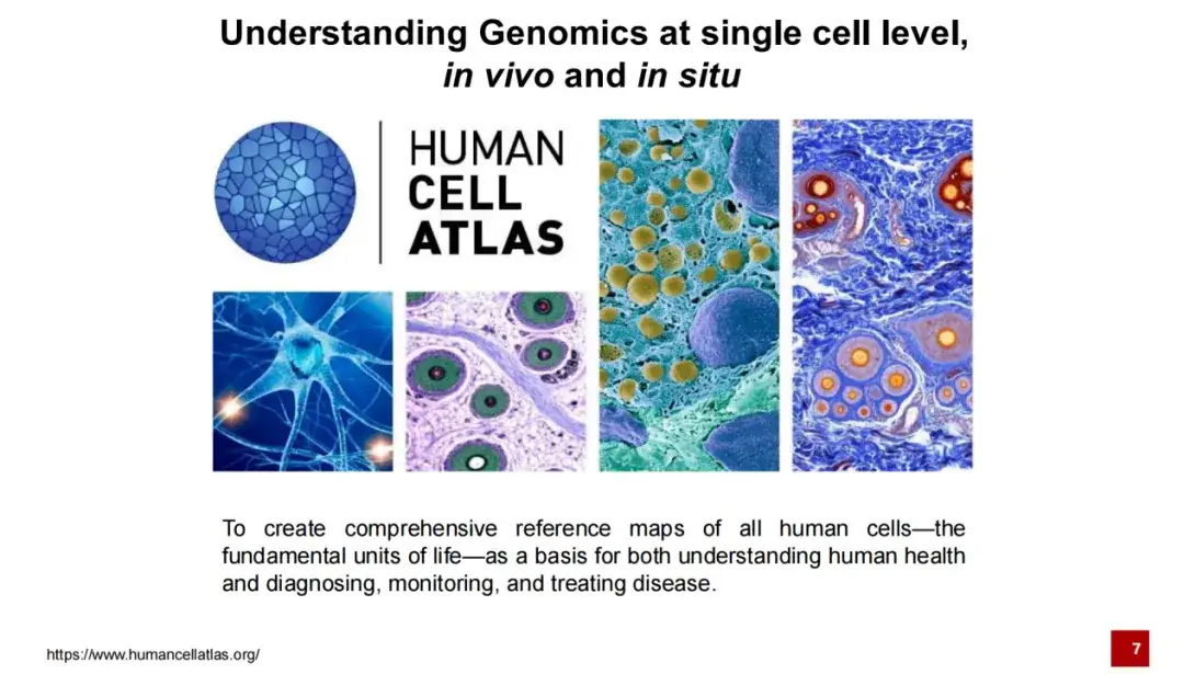
Since the launch of the Human Genome Project until the proposal of the Human Cell Atlas Project in 2016, its goal has been to complete the reference map of all human cells to help us better understand life activities and provide support for the treatment and diagnosis of specific diseases.

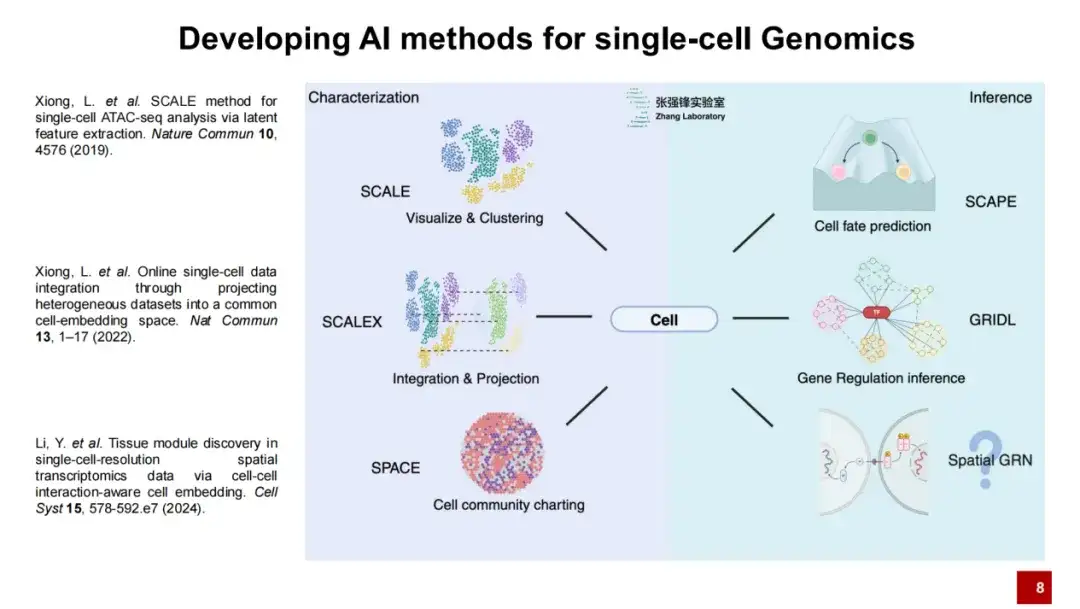
The team developed three methods: SCALE, SCALEX and SPACE for single-cell genomics research

Our lab has developed a series of artificial intelligence methods.We believe that single-cell genomics requires two major steps: first, the description of the cells, and second, the inference of the cells.

We have published three works to describe cells: SCALE, SCALEX and SPACE.SCALE is mainly for visualization and clustering, SCALEX is for data integration and projection, and SPACE is for the description of the microenvironment of the entire spatial transcriptome data organization.Today I will mainly introduce the two methods: SCALEX and SPACE.

SCALEX method to eliminate batch effects

The SCALEX method is to eliminate batch effects.This is a very important issue in genomic research. Batch effect refers to the differences in experimental results between different batches due to technical factors such as different experimental conditions.

As shown in the figure below, even if we culture two groups of biologically replicated cells separately, theoretically sequencing these two groups of cells should yield very similar gene expressions. However, due to technical reasons, such as differences in culture environment, library construction time, or sequencing platform,The final gene expression profiles may vary greatly, thus introducing a lot of technical noise.Therefore, when analyzing the data, it is necessary to remove this batch effect.

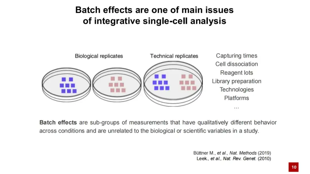
In biological research, data cannot be collected all at once, but is accumulated gradually through multiple experiments.Remove batch effects and analyze data in an integrated manner to find factors that are truly biologically relevant.It is a key step in genomics or single-cell genomics research.

Based on this, we developed the SCALEX method.It is able to project the processed single-cell data into a generalized cellular latent space. The framework of SCALEX is based on variational autoencoders (VAE).

The first input is the transcriptome data of a single cell, which is then projected into a generalized cellular latent space through a batch-free encoder.

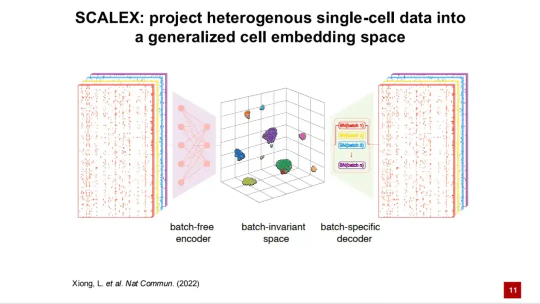
Then, the batch information is added to the model through domain-specific batch normalization through a batch-specific decoder. Through this asymmetric design, the generated cell latent space is a batch-independent space, which theoretically does not contain any batch-related technical noise. The gene expression is reconstructed through the decoder, and the loss is calculated with the original input gene expression spectrum. At the same time, the KL divergence is combined to form the loss function of the SCALEX model, which is a self-supervised model.

This asymmetric encoder and decoder design has two main advantages:First, the resulting encoder is universal.That is, new data can be directly projected into the cell latent space without batch information through the encoder without retraining the model or reintegrating the new data into the existing data.

Second, SCALEX pays more attention to the global batch effect.The traditional method of removing batch effects is mainly to find similar cells (cell pairs) in two batches of data and pair them for correction to remove the batch effect. This method is essentially a relatively local batch effect correction.

However, there is a problem with this type of method. In actual data analysis, the cell types in two different batches may not be completely consistent. There may be only a few cell types in common, and the rest are batch-specific. If you forcefully search for cell pairing, it may be impossible to find suitable paired cells, resulting in over-correction, and forcibly aligning cell types that should not be aligned.

In this regard, I will explain the two major advantages of SCALEX in more detail.

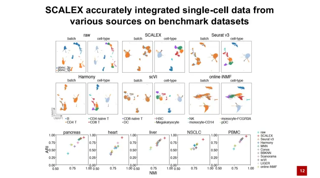
First, we benchmark SCALEX on five test datasets.The results show that SCALEX outperforms existing methods in terms of accuracy.

As shown in the figure below, the batch graph represents the original and uncorrected data, blue and orange represent the data of two batches, and cell-type represents the cell type. It can be seen that although there are similar cell types in these two batches, due to the large batch effect, cells that originally belonged to the same cell type cannot be aggregated together, resulting in technical factors covering up biological factors and making subsequent biological research impossible.

After SCALEX integration, the two batches of cells were able to aggregate well together and were clearly separated according to cell types, demonstrating the importance of SCALEX in practical applications.

An important advantage of SCALEX is that it can process two batches of data with the same cell types.This kind of data is called partial overlapping datasets. As shown in the figure below, overlap 0 means that the cell types in the two batches are completely different, and overlap 4 means that there are 4 shared cell types in the two batches.

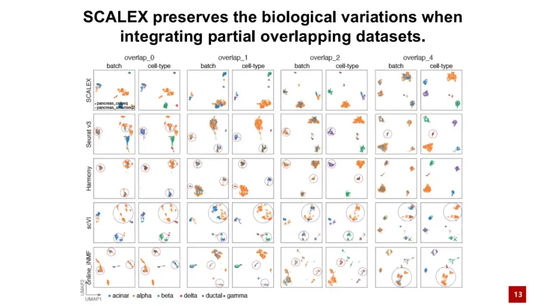
The results show that even when the two batches of cells have no identical cell types at all, SCALEX can still maintain biological differences well, that is, SCALEX will not forcibly integrate cells of different cell types together, while other similar methods may rely on finding cell pairings, resulting in over-correction.
Another advantage of SCALEX is that the universal encoder can directly project new data into the existing latent space of cells without batch effects, without retraining the model.As shown in the figure below, a reference cell atlas is first trained using the pancreas datasets, and then three new data are directly projected into the cell latent space through the trained encoder. The colors in the figure represent the cell types, and the gray dots represent the constructed reference cell types. It can be seen that the positions of different cell types in the figure are well separated.

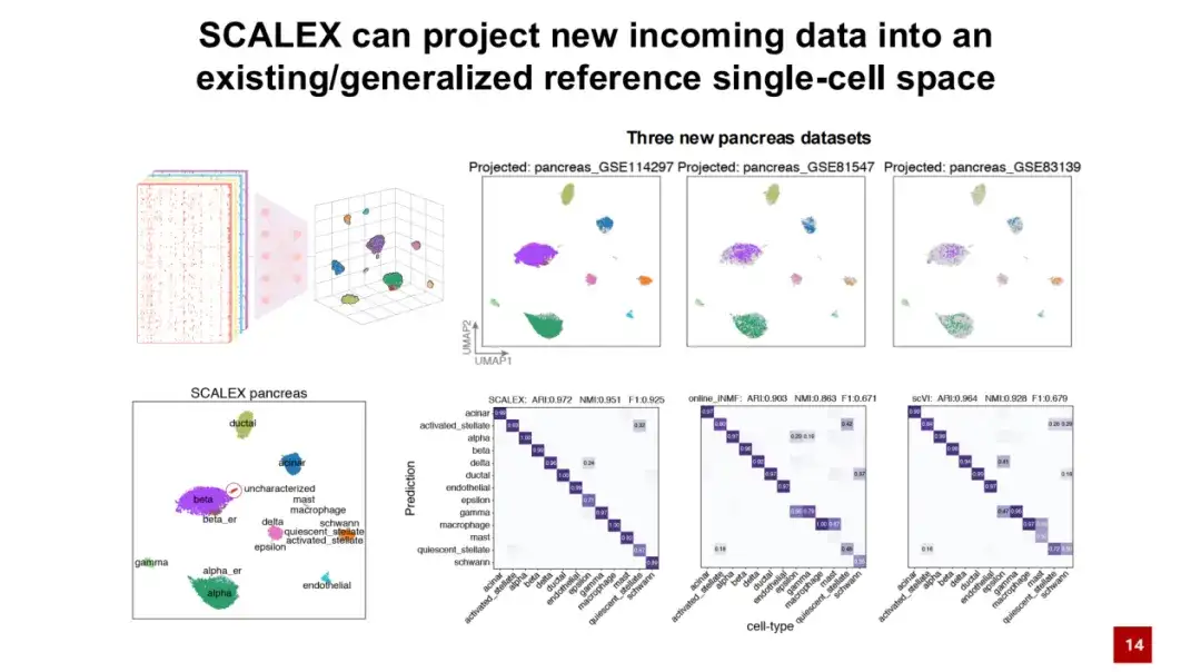
By projecting the labels of reference cells around a specific location onto new data cells, we can see that SCALEX performs well in automatically annotating cell types. Compared with other existing methods, SCALEX has a very important application.That is, new data can be directly projected into the constructed data, helping us to conduct comparative analysis between data.

In addition, SCALEX also performs well in processing large-scale data. The figure below shows that when SCALEX processes 4 million cell data, the calculation time does not exceed tens of minutes and the memory consumption is less than 100 GB. This shows that SCALEX has good scalability and can be used for integrated analysis of ultra-large-scale single-cell data.

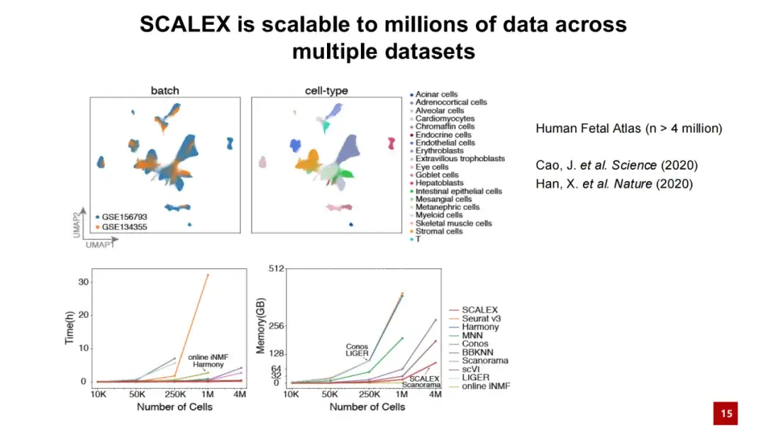
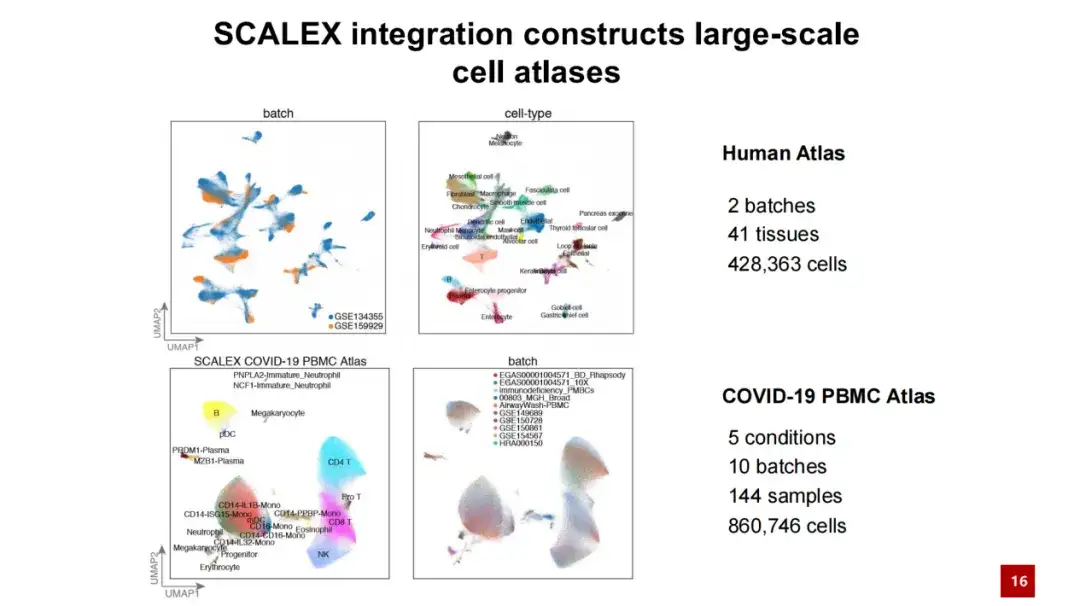
Taking advantage of SCALEX, we have constructed two large-scale cell atlases, one is a cell atlas of human individuals, containing more than 400,000 cells; the other is a COVID-19 PBMC cell atlas, containing more than 860,000 cells and more than 100 samples.

SPACE: an artificial intelligence analysis tool for spatial transcriptome data

Next, I will introduce to you the spatial transcriptome analysis tool SPACE that my team recently published.

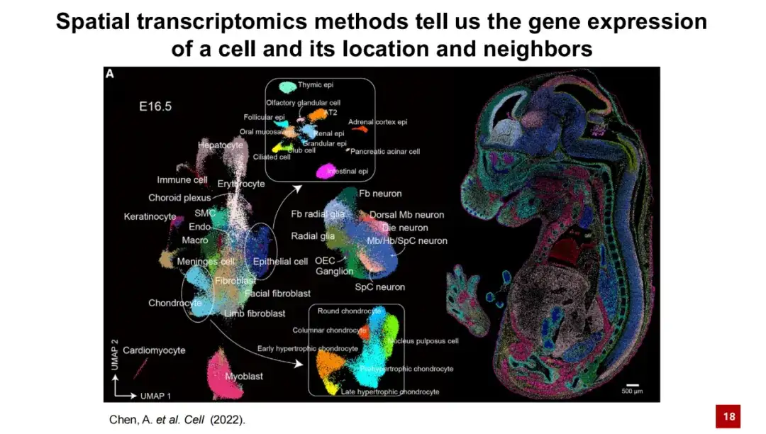
In simple terms, spatial transcriptome technology can provide gene expression information of cells and their specific location in space. The figure below shows a typical spatial transcriptome result. In the left figure, each point represents a cell, and the color indicates its cell type. These cells form a UMAP graph through dimensionality reduction clustering of gene expression. In the right figure, the actual spatial position of each cell in the mouse embryo E16.5 data is shown. It can be clearly seen that the spatial distribution of cells has good specificity.

Organization research has always been one of the core issues in life science research. It can be said that one of the long-term goals of biological research is to understand the relationship between the structure of an organization and its function. This is easy to understand. For example, different brain regions in the brain are composed of different neurons and supporting cells, and perform different functions through complex cell-to-cell interactions. For example, some regions are responsible for memory, some are responsible for learning, and some are responsible for motor response.

therefore,A core issue in spatial transcriptome analysis is to identify different cell types or tissue modules in space, a task collectively referred to as spatial clustering.

This task consists of two subtasks: one is to identify the cell type, and the other is to identify the tissue module.The former is more intuitive, i.e. identifying various cell types in spatial transcriptome data, such as shown in mouse embryo data; while the latter is relatively abstract, involving the identification of regions within the tissue that are smaller than the tissue structure, which may have specific functions or be composed of cells.

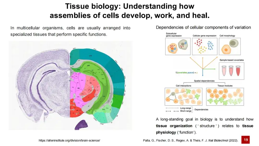
In different studies, researchers give different names to tissue modules, such as spatial domain or cell niche, among which spatial domain is a more commonly used term. Some researchers believe that identifying tissue modules is to identify regions with consistent spatial gene expression characteristics.

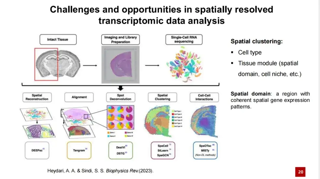
However, this concept has limitations. For example, Figure A below shows that there is a significant difference in gene expression between two regions, but in Figures B and C, the gene expression distribution between regions is not completely clean and may be mixed. Figures B and C show situations that the spatial domain concept cannot solve.

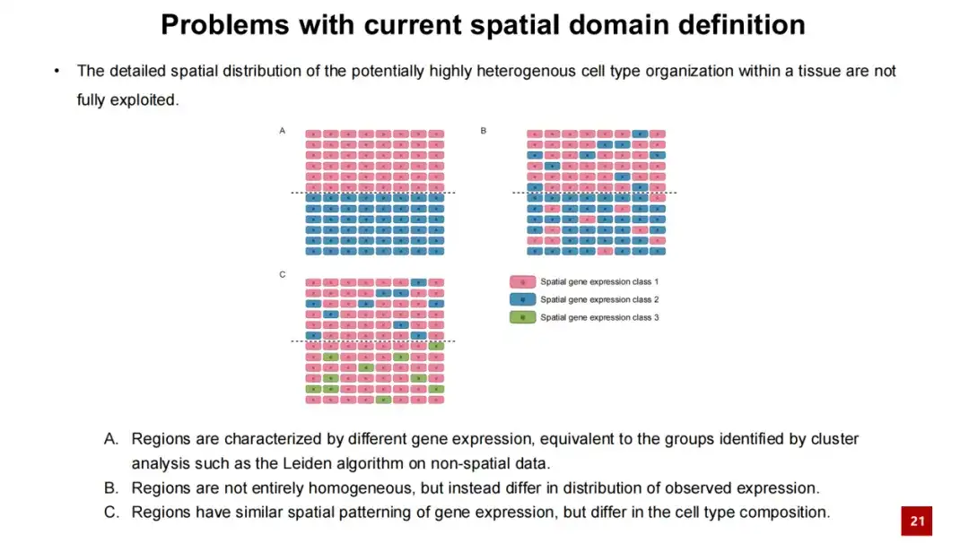
To address this problem, we propose the SPACE method.The spatial domain problem is addressed by learning interaction-aware cell embeddings.

SPACE uses a graph autoencoder framework to learn low-dimensional cell embeddings.

First, we input the spatial transcriptome data and construct a neighboring graph based on the spatial position of each cell, that is, connect the nearest neighbor cells of each cell to form a graph. In the figure below, the nodes represent cells, and the features of the nodes are the gene expression features of the cells. We input the neighboring graph and gene expression profiles into the encoder of SPACE, which consists of a three-layer GAT network.

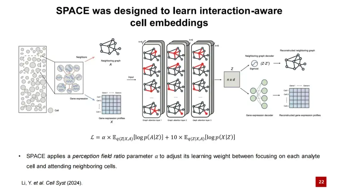
Through the processing of the encoder, we can obtain the embedded representation of each node and reconstruct it through two independent decoders:One decoder reconstructs the low-dimensional cell hidden layer representation back into a neighborhood graph, while the other decoder reconstructs the gene expression profile of the cell. The loss function of the SPACE model is the sum of these two reconstruction losses.

In this process,We design a perception field ratio parameter α to adjust the weights of the two loss functions in the model.

When the α value is small,The model focuses more on reconstructing the gene expression of the cell itself, and the cell embedding obtained can be used to identify the cell type;When the α value is large,The model focuses more on the interaction between cells, and the cell embeddings obtained at this time can be used to identify tissue modules. Because the low-dimensional cell embedding Z contains information about cell interactions, we call the low-dimensional embedding representation obtained by SPACE interaction-awara cell embeddings.

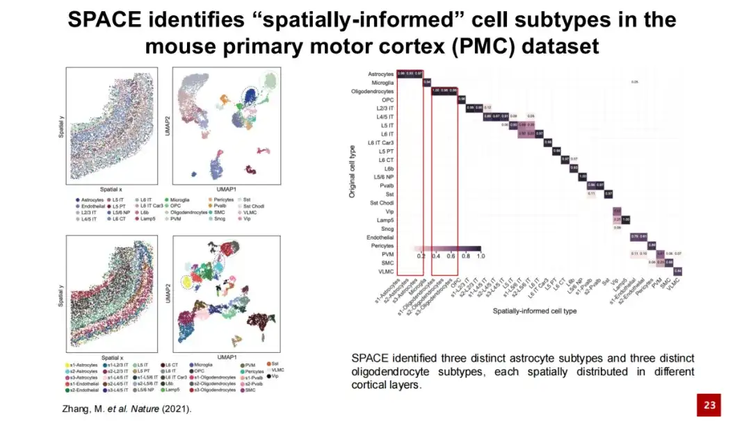
To identify spatial cell subtypes, we applied SPACE to the mouse primary motor cortex dataset.

In the figure below, the upper left figure shows the spatial position of each cell in the actual tissue, where a dot represents a cell and the color indicates the cell type. This is a UMAP map generated based on gene expression. The two figures on the lower left show the spatial cell subtypes identified by SPACE and their positions in space. We performed a confusion matrix analysis on these spatial cell subtypes and the cell types provided in the original study (as shown in the figure on the right), and the results showed that the two were generally consistent, with an adjusted Rand Index (ARI) of 0.6. At the same time, SPACE can differentiate astrocytes from oligodendrocytes more finely and identify more cell subtypes.

The lower left image shows the organizational structure of the primary motor cortex of mice. Layer represents the cortical structure and WM represents White Matter. The layered structure from Layer 1 to White Matter can be clearly seen. The three astrocyte subtypes identified by SPACE are difficult to distinguish only by gene expression, and they are mixed together in the UMAP map.

However, these three cell subtypes are clearly distinguished in spatial distribution: s1 cell subtype is mainly distributed in the area from Layer 1 to Layer 4, s2 is mainly distributed in the area from Layer 5 to Layer 6, and s3 is mainly distributed in White Matter. We counted the proportions of cell types around these three stellate cell subtypes, and the results were consistent with this stratification rule. Although these three cell subtypes are similar in gene expression, they still show their own specific high-expression genes.

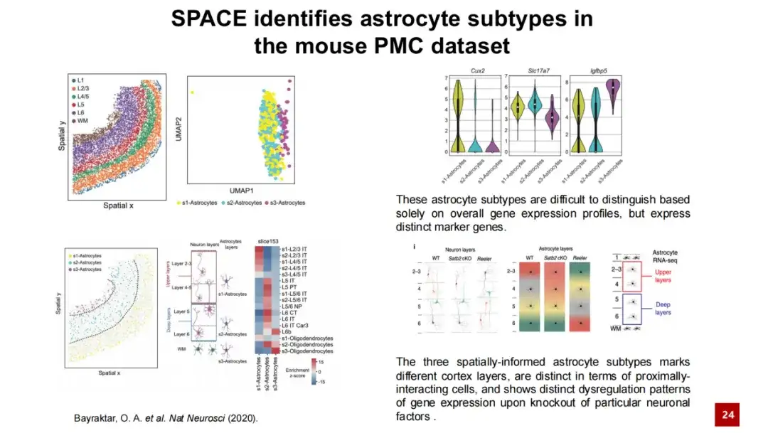
The three stellate cell subtypes identified by SPACE are highly consistent with previous studies. Previous studies have reported that there is an interaction between stellate cells and neurons, and the stratification of stellate cells corresponds to the stratification of neurons. By knocking out key factors in neurons, the researchers found that the stratified structure of neurons was destroyed, and the stratified structure of stellate cells also changed accordingly. This indicates that there is a spatially specific interaction and spatially specific gene regulation between stellate cells and neurons.

From this example we can see thatSPACE can effectively utilize spatial information and accurately identify different biological cell types with spatial characteristics.

The previous article introduced that SPACE changes the optimization direction of the model by adjusting the perception field ratio parameter α: it can pay more attention to the characteristics of the cells themselves to identify cell types, or pay more attention to the interaction information between cells to discover tissue modules.

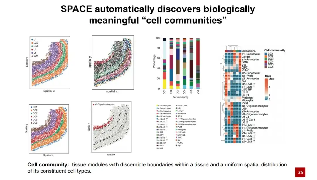
In the same dataset,By increasing the α value, SPACE successfully discovered the tissue module.We named them Cell Communities (CC). We believe that the tissue modules discovered by SPACE have recognizable boundaries, and the spatial distribution of cell types within them is relatively uniform and consistent. We compared the cell communities discovered by SPACE with existing tissue structures and found that the two have a good one-to-one correspondence. Each cell community contains different cell types, and the spatial distribution of these cell types within the cell community is relatively uniform.

We compared SPACE with existing methods for discovering organizational modules and conducted tests on five datasets.The results show that SPACE outperforms the best existing methods in 2 datasets and performs comparable to the best methods in the other 3 datasets.We also conducted tests and analyses on the commonly used Visium human brain dataset, and the results showed that SPACE is also applicable to spatial transcriptome data without single-cell resolution.

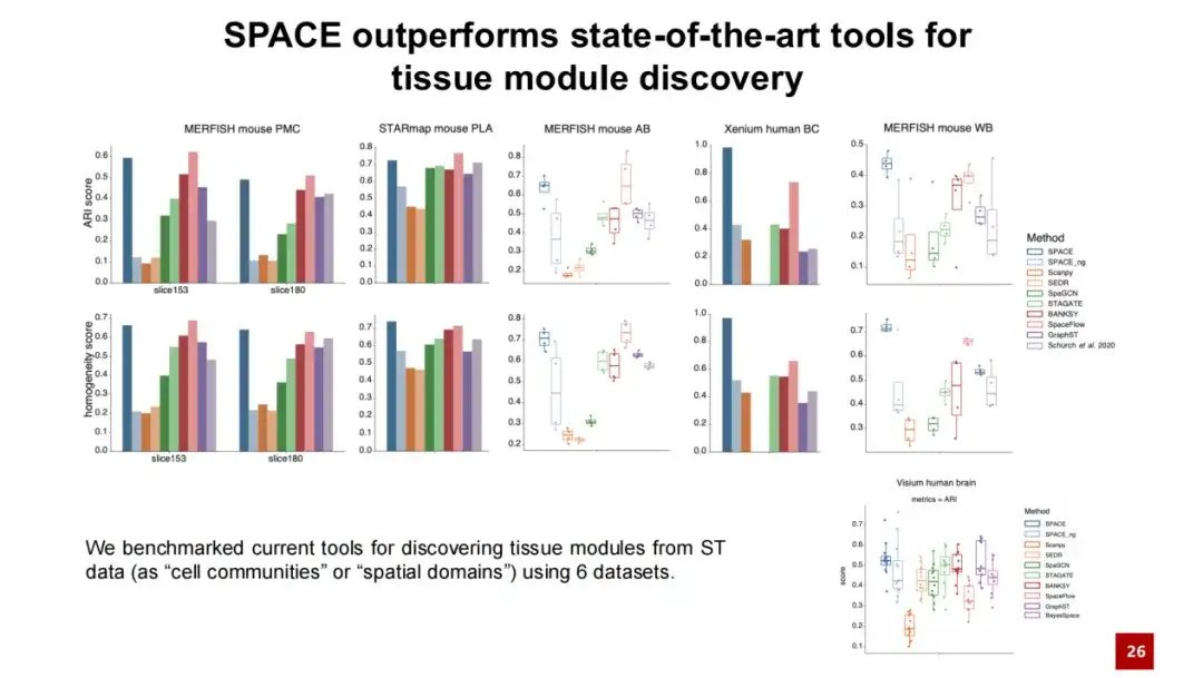
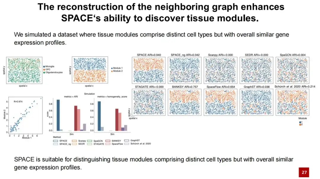
In addition, we introduced a test model named SPACE_ng, where ng means we turned off the neighbor graph reconstruction loss in the SPACE model. The results show that the performance of SPACE_ng is far inferior to SPACE.

To further illustrate that SPACE's ability to discover organizational modules well comes from the reconstruction of the neighbor graph, we designed a simulation experiment. We selected oligodendrocytes and evenly distributed microglia and OPC cells among the oligodendrocytes (see the upper left figure below), forming two organizational modules.

Since most of the cells in these two tissue modules are oligodendrocytes and have a very high similarity (collaboration = 0.97), the test results show that SPACE is far superior to other methods, while SPACE_ng cannot distinguish between the two tissue modules.This indicates that the performance of the SPACE tissue recognition module stems from its reconstruction of the neighborhood graph.

We observed a similar phenomenon in downstream analysis, that is, the characteristics of cell communities identified by SPACE are not simply manifested as consistent spatial gene expression as in spatial domains, but reflect similar interactions between neighboring cells.

In the heat map below, each column represents a cell, and its color indicates the cell population to which the cell belongs and its cell type. Each row represents a cell type, showing the relative frequency of neighbor interactions between that cell type and other cells. From this heat map, we can see that cells belonging to the same cell population show similarities in neighbor interactions, and this similarity is independent of the specific cell type. In contrast, cells belonging to different cell populations have large differences in neighbor interactions.

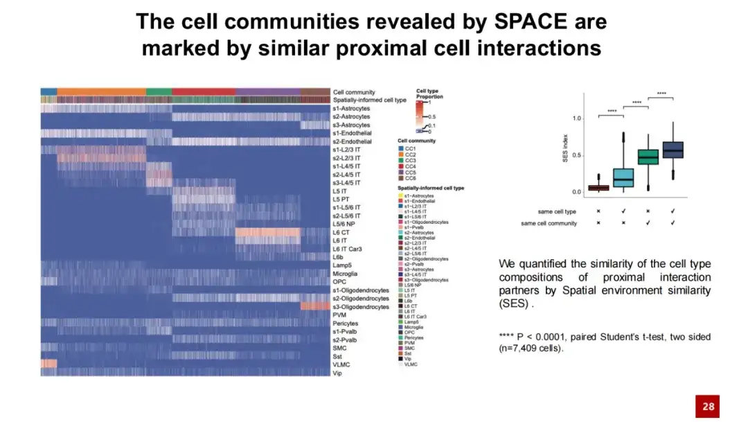
We further quantitatively calculated the similarity of cell-cell interactions using cosine similarity. The results showed that cells from the same cell population had high similarity in their interactions with neighboring cells, while cells from different cell populations had relatively different extracellular interactions. These results indicate thatThe cell communities discovered by SPACE are not just a spatial gene expression pattern, but are also influenced by the proximal cell interaction network.

We performed a similar analysis in another mouse placenta dataset. The left image shows the spatial location of each cell type in the dataset, the middle left image shows the manually annotated mouse placenta tissue structure, and the middle right image shows the five cell populations discovered by SPACE. It can be seen that there is a good one-to-one correspondence between the cell populations discovered by SPACE and the manually annotated tissue structures. We constructed a characteristic proximal cell interaction network for each cell population, as shown in the right image, showing the unique cell-to-cell interactions within each cell population.

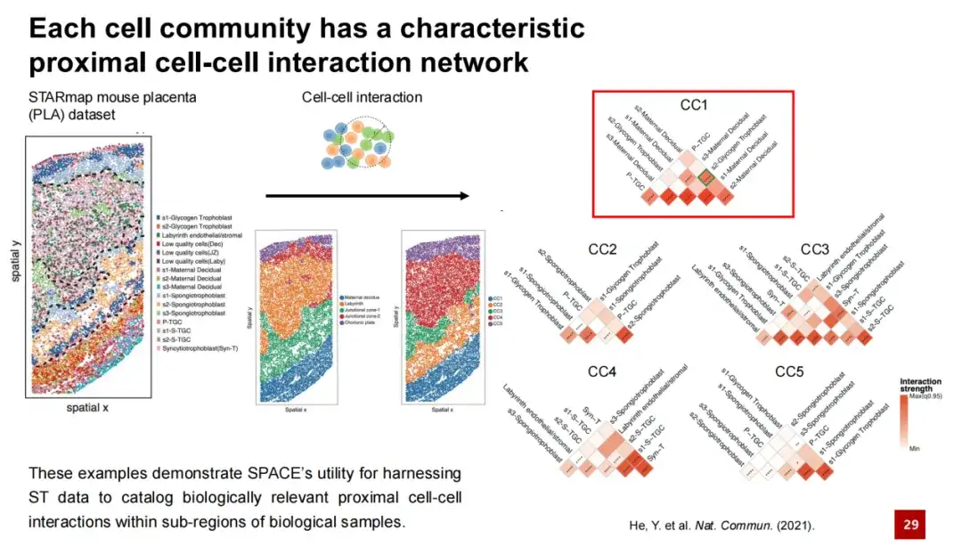
Taking CC1 as an example, this community is mainly located in the maternal decidua region. We found that in CC1, there is a strong interaction between s2 maternal decidua cells and s2 glycotrophoblasts. Previous studies have shown that during mouse pregnancy, glycotrophoblasts invade the maternal decidua region and interact with maternal decidua cells therein, thereby initiating the remodeling process of the arteries that bring maternal blood into the placenta, which is essential for normal pregnancy.

From the above analysis, we can conclude thatSPACE can identify cell-cell interactions in biological samples that have important impacts on life processes.Therefore, we speculate thatThe interaction networks constructed by SPACE can be used to optimize ligand-receptor based cell communication analysis.

Ligand-receptor-based cell communication analysis is a common method in single-cell data analysis, which is to infer the possibility of cell communication between two cells through ligand-receptor pairs based on the gene expression of their ligands and receptors. We first analyzed the intercellular communication in CC1 using CellChat (a commonly used cell communication analysis method) in the mouse placenta dataset.

CellChat found that s3 maternal decapping cells can communicate with P-TGC cell types through signaling pathways such as collagen FN1 and THBS. However, these signaling pathways require physical contact to actually occur. But we found that the two cell types are actually far apart in spatial distribution (see the lower right corner of the figure below), and it is unlikely that they will actually have physical contact.

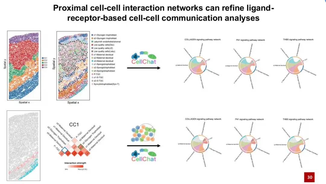
This is also confirmed by the proximal cell interaction network constructed in CC1. The blue boxes show that they are unlikely to interact with each other.Introducing the characteristic proximal cell interaction network constructed by SPACE into CellChat cell communication analysis can help us exclude cell communication signals that are actually impossible to occur in space, thereby effectively reducing false positive signals.

Careers

Tsinghua University and the State Key Laboratory of Membrane Biology have established a branch of membrane structure and artificial intelligence biology in HangzhouCurrently, the team is recruiting professionals who are engaged in research at the intersection of artificial intelligence and biology. We sincerely invite researchers who are interested in this field to join the team. For more information about the recruitment, please scan the QR code below for more information.