Command Palette
Search for a command to run...
PipeTransformer: Automated Elastic Pipeline for large-scale Distributed Model Training
Paper title:
PipeTransformer: Automated Elastic Pipelining for Distributed Training of Large-scale Models
Pipetransformer uses automated elastic pipelines to perform efficient distributed training of Transformer models. In PipeTransformer, we designed an adaptive dynamic freezing algorithm that can gradually identify and freeze certain layers during training, and designed an elastic pipeline system that can dynamically allocate resources to train the remaining active layers.
Specifically, PipeTransformer automatically excludes frozen layers from the pipeline, packs active layers into fewer GPUs, and branches more replicas to increase data parallel width.
Evaluations on ViT (using the ImageNet dataset) and BERT (using the SQuAD and GLUE datasets) show that PipeTransformer achieves up to 2.83x speedup compared to the state-of-the-art baselines without any loss in accuracy.
The paper also includes a variety of performance analyses to help users gain a more comprehensive understanding of the algorithm and system design.
Next, this article will introduce in detail the research background, motivation, design ideas, design solutions of the system, and how to implement the algorithm and system using PyTorch distributed API.
Introduction

Large Transformer models have achieved accuracy breakthroughs in both natural language processing and computer vision. GPT-3 has set new high-precision records for most NLP tasks. In ImageNet, Vision Transformer (ViT for short) also achieved a top-1 accuracy of 89%, outperforming the most advanced convolutional networks ResNet-152 and EfficientNet.
To address the problem of ever-increasing model sizes, researchers have proposed various distributed training techniques, including parameter servers, pipeline parallelism, intra-layer parallelism, and zero redundancy data-parallel.
However, existing distributed training solutions are only research scenarios, and all model weights must be optimized during training (i.e., the computation and communication overhead must remain relatively stable during different iterations). Recent research on progressive training shows that the parameters in neural networks can be trained dynamically:
- Singular Vector Canonical Correlation Analysis for Deep Learning Dynamics and Interpretability. NeurIPS 2017
- Efficient Training of BERT by Progressively Stacking. ICML 2019
- Accelerating Training of Transformer-Based Language Models with Progressive Layer Dropping. NeurIPS 2020
- On the Transformer Growth for Progressive BERT Training. NACCL 2021

Figure 2: Interpretable frozen training: DNN bottom-up convergence (using ResNet to test results on CIFAR10) Each pane shows the similarity of each layer through SVCCA
For example, in frozen training, neural networks typically converge bottom-up (i.e., not all layers need to be trained to achieve some result).
The figure above shows an example of how weights gradually stabilize during training with a similar approach.We leverage frozen training to perform distributed training of Transformer models, which accelerates training by dynamically allocating resources to focus on a reduced set of active layers.
This layer freezing strategy is particularly suitable for pipeline parallelism, because excluding consecutive bottom layers from the pipeline can reduce computation, memory, and communication overhead.
Figure 3: PipeTransformer’s automated and flexible pipeline process accelerates distributed training of Transformer models
PipeTransformer is a flexible pipeline training acceleration framework that automatically reacts to frozen layers by dynamically transforming the scope of pipeline models and the number of pipeline replicas.
To the best of our knowledge, this is the first paper to study layer freezing in the context of pipeline and data-parallel training.
Figure 3 illustrates the advantages of this combination.
First, by excluding frozen layers from the pipeline, the same model can be packed into fewer GPUs, resulting in less cross-GPU communication and smaller pipeline bubbles.
Second, after packing the model onto fewer GPUs, the same cluster can accommodate more pipeline replicas, thereby increasing the width of data parallelism.
More importantly, the two advantages are multiplicative rather than additive, thus further speeding up training progress.
The design of PipeTransformer faces four major challenges.
First, the freezing algorithm must make dynamic and adaptive freezing decisions; however, existing work only provides a post hoc analysis tool.
Second, the efficiency of pipeline repartitioning is affected by many factors, including partition granularity, cross-partition activation size, and the number of mini-batch chunks, which requires reasoning and searching in a larger solution space.
Next, to dynamically introduce additional pipeline replicas, PipeTransformer must overcome the static nature of collective communication and avoid potentially complex cross-process messaging protocols (a pipeline can only be handled by one process) when new processes come online.
Finally, the cache can save time for repeated forward propagation of frozen layers, but it must be shared between existing pipelines and newly added pipelines because the system cannot create and warm up a dedicated cache for each replica.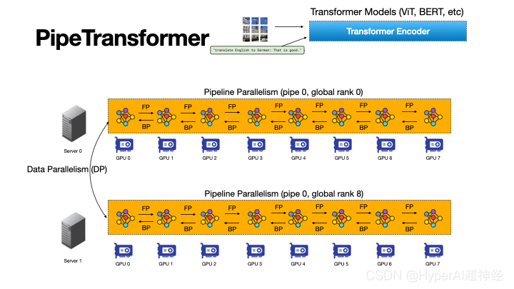
Figure 4: PipeTransformer Dynamics diagram
As shown in Figure 4, in order to meet the above challenges,The design of PipeTransformer consists of four core building blocks.
First, there is a tunable adaptive algorithm that generates signals that guide the selection of frozen layers in different iterations (freezing algorithm). Once triggered by these signals, the elastic pipeline module (AutoPipe) packs the remaining active layers into fewer GPUs by evaluating the changes in the activity size and workload of heterogeneous partitions (frozen and active layers).
Next, based on the previous analysis results of different pipeline lengths, a mini-batch is decomposed into a series of better micro-batches.
The next module, AutoDP, generates additional pipeline copies to occupy the released GPUs and maintains hierarchical communication process groups to achieve dynamic membership for collective communication.
The last module, AutoCache, efficiently shares activations between existing and newly added data-parallel processes and automatically replaces stale cache during transformations.
In general, PipeTransformer combines the freezing algorithm, AutoPipe, AutoDP, and AutoCache modules to provide significant training acceleration.
We evaluate PipeTransformer with ViT (using the ImageNet dataset) and BERT (using the SQuAD and GLUE datasets) models and show that PipeTransformer achieves up to 2.83x speedup compared to the state-of-the-art baselines without any loss in accuracy.
We also provide various performance analyses to help users more fully understand the algorithmic and systemic design. Finally, we have developed an open source, flexible API for PipeTransformer that clearly separates freezing algorithms, model definition, and training acceleration, allowing migration to algorithms that require similar freezing strategies.
Overall Design
Suppose our goal is to train a large-scale model in a distributed training system. This system combines pipeline model parallelism and data parallelism and can be used to handle the following scenarios:
The model cannot fit into the memory of a single GPU device, or the batch size is small when loading to avoid running out of memory. Specifically, the settings defined are as follows:
- Training tasks and model definitions. Train Transformer models (such as Vision Transformer, BERT, etc.) on large-scale image or text datasets. The Transformer model mathcalF has a total of L layers, where the i-th layer consists of a forward calculation function fi and a set of corresponding parameters.
- Training infrastructure. Assume that the training infrastructure consists of a GPU cluster with N GPU servers (i.e. nodes). Each node has I GPUs. The cluster is homogeneous, which means that the hardware configuration of each GPU and server is the same. The memory capacity of each GPU is MGPU. The servers are connected to each other via high-bandwidth network interfaces (such as InfiniBand).
- Pipeline parallelism. In each machine, we load a model F into a pipeline with K partitions (K also represents the pipeline length). The kth partition consists of Pk consecutive layers. Assume that each partition is processed by a GPU device. 1≤K≤I means that we can build multiple pipelines for multiple model copies on a single device.
Assume that all GPU devices in a pipeline belong to the same machine, the pipeline is synchronous, no expired gradients are involved, and the number of micro-batches is M. In the Linux operating system, each pipeline is handled by a process. For more details, please refer to GPipe.
- Data parallelism. DDP is a cross-machine distributed data parallel processing group inside R parallel workers. Each worker is a pipeline replica (single process). The index (ID) of the rth worker is rank r.
For any two pipelines in DDP, they can belong to the same GPU server or different GPU servers, and can also exchange gradients with the AllReduce algorithm.
In these cases, our goal is to speed up training by taking advantage of frozen training, which eliminates the need to train all layers during the entire training process.
In addition, this helps save computation, communication, and memory loss, and avoids overfitting caused by continuous freezing of layers to a certain extent.
However, to take advantage of these advantages, the four challenges mentioned above must be overcome, namely designing an adaptive freezing algorithm, dynamic pipeline repartitioning, efficient resource reallocation, and cross-process caching.
Figure 5: Overview of the PipeTransformer training system
PipeTransformer co-designs an instant freezing algorithm and an automatic elastic pipeline training system that can dynamically convert the scope of the pipeline model and the number of pipeline replicas. The overall system architecture is shown in Figure 5.
To support the elastic pipeline of PipeTransformer, we maintain a customized version of PyTorch Pipeline. For data parallelism, we use PyTorch DDP as a baseline. Other libraries are standard mechanisms of the operating system (such as multi-processing), which also eliminates the need for customization of software or hardware.
To ensure the versatility of the framework, we decouple the training system into four core components: freezing algorithm, AutoPipe, AutoDP, and AutoCache.
The freezing algorithm (grey) samples metrics from the training loop and makes layer-by-layer freezing decisions, which are shared with the AutoPipe (green).
AutoPipe is a flexible pipeline module that speeds up training by excluding frozen layers from the pipeline and packing active layers onto fewer GPUs (pink), thereby reducing cross-GPU communication and keeping pipeline stalls smaller.
AutoPipe then passes the pipeline length information to AutoDP (purple), which then generates more pipeline copies when possible to increase the width of data parallelism.
The figure also includes an example where AutoDP introduces a new replica (in purple). AutoCache (in orange) is a cross-pipeline cache module. For readability and generality, the source code architecture remains the same as Figure 5.
Implementation using PyTorch API
As can be seen from Figure 5, PipeTransformer consists of four components: Freeze Algorithm, AutoPipe, AutoDP and AutoCache.
Among them, AutoPipe and AutoDP depend on PyTorch DDP (torch.nn.parallel.DistributedDataParallel) and pipeline (torch.distributed.pipeline) respectively.
In this blog, we only highlight the key implementation details of AutoPipe and AutoDP. For more information on the freezing algorithm and AutoCache, please refer to the paper.
AutoPipe: Flexible Pipeline
AutoPipe can speed up training by excluding frozen layers from the pipeline and compressing active layers onto fewer GPUs.This section details the key components of AutoPipe:
1) Dynamic partition pipeline;
2) Reduce the number of pipeline equipment;
3) Optimize mini-batch chunk size accordingly
Basic usage of PyTorch pipeline
Before delving into the details of AutoPipe, let's first get familiar with the basic usage of PyTorch Pipeline (torch.distributed.pipeline.sync.Pipe):
To understand pipeline design in action, consider the following simple example:
# Step 1: build a model including two linear layers
fc1 = nn.Linear(16, 8).cuda(0)
fc2 = nn.Linear(8, 4).cuda(1)

# Step 2: wrap the two layers with nn.Sequential
model = nn.Sequential(fc1, fc2)

# Step 3: build Pipe (torch.distributed.pipeline.sync.Pipe)
model = Pipe(model, chunks=8)

# do training/inference
input = torch.rand(16, 16).cuda(0)
output_rref = model(input)
In this simple example, you can see that before initializing Pipe, you need to partition the nn.Sequential model into multiple GPU devices and set the optimal number of chunks.
Balancing the computations across partitions is critical to pipeline training speed, as uneven distribution of workloads across stages can cause lags, forcing devices with fewer tasks to wait. The number of chunks can also have a significant impact on pipeline throughput.
Balancing pipeline partitions
In dynamic training systems such as PipeTransformer, simply having the same number of parameters in each partition does not guarantee the fastest training speed. Other factors also play a key role:
Figure 6: The partition boundary is located in the middle of the skip connection
1. Cross-partition communication overhead. Placing the partition boundary in the middle of a skip connection results in extra communication because tensors in the skip connection must then be copied to different GPUs.
For example, for the BERT partitions in Figure 6, partition k must obtain intermediate outputs from partition k-2 and partition k-1. In contrast, if the boundary is placed after the addition layer, the communication overhead between partition k-1 and partition k becomes significantly smaller.
Measurements show that cross-device communication is more expensive than slightly unbalanced partitions, so we do not consider breaking skip connections.
2. Freeze layer memory usage. During training, AutoPipe must recalculate partition boundaries several times to balance two different types of layers: frozen layers and active layers.
Given that frozen layers do not require backward activation maps, optimizer states, and gradients, the memory cost of frozen layers is only a fraction of that of inactive layers.
Instead of launching an intrusive profiler to get the underlying metrics of memory and compute costs, we define a tunable cost factor lambdafrozen to evaluate the memory usage of a frozen layer relative to the same active layer. We set it to 1/6 based on empirical measurements on our experimental hardware.
Based on the above two points, AutoPipe can balance pipeline partitions according to parameter sizes.Specifically, AutoPipe uses a greedy algorithm to allocate frozen layers and active layers so that the sub-layers of the scoring region can be evenly distributed to K GPU devices.
The pseudocode is the load_balance() function in Algorithm 1. The frozen layers are extracted from the original model and saved in a separate model instance Ffrozen in the first device of the pipeline.
Note that the segmentation algorithm used in this article is not the only option;PipeTransformer is modular and can be run in conjunction with any of the alternatives.
Pipeline compression
Pipeline compression helps free up the GPU to accommodate more pipeline copies and reduces the amount of cross-device communication between partitions. To determine how long to compress, we can estimate the memory consumption of the largest partition after compression and then compare it to the memory consumption of the largest partition of the pipeline at timestep T=0.
To avoid extensive memory profiling, the compression algorithm uses parameter size as a proxy for training memory usage. Based on this simplification, the guidelines for pipeline compression are as follows: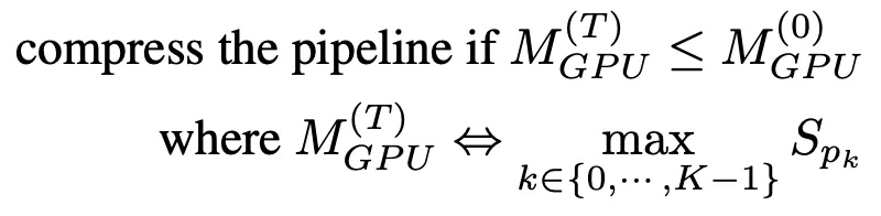
Once a freeze notification is received, AutoPipe attempts to divide the pipeline length K by 2 (for example, from 8 to 4, then 2). By inputting K/2, the compression algorithm can verify whether the compression result meets the criteria in formula (1).
The pseudo code is shown in lines 25-33 of Algorithm 1. Note that this compression makes the speedup grow exponentially during training, which means that if a GPU server contains more GPUs (for example, more than 8), the speedup will increase further. Figure 7: Pipeline Bubble
Fd, b and Ud represent the forward, backward and optimizer updates of micro=batch b on device d, respectively.
The total bubble size in each iteration is K-1 times the forward and backward cost per micro=batch.
In addition, this technique can also speed up training by reducing the size of the Pipeline Bubble. To explain the bubble size in the pipeline, Figure 7 describes how 4 micro-batches run through 4 device pipelines with K=4.
In general, the total bubble size is K-1 times the forward and backward cost per micro-batch. Therefore, it is obvious that shorter pipelines have smaller bubble sizes.
Dynamic Number of Micro-Batch
Previous pipeline parallel systems used a fixed number of micro-batches per mini-batch (M). GPipe recommends M ≥ 4 x K, where K is the number of partitions (pipeline length). However, given that PipeTransformer dynamically configures K, we found that keeping M static during training does not work well.
In addition, when integrated with DDP, the value of M also affects the efficiency of DDP gradient synchronization. Since DDP must wait for the last micro-batch to complete the backward calculation of a parameter before gradient synchronization, the finer the micro-batch, the smaller the overlap of computation and communication.
Therefore, PipeTransformer does not use static values, but dynamically searches for the optimal value of M in the hybrid of the DDP environment by enumerating the values of M in the range of K-6K. For a specific training environment, profiling only needs to be completed once (see Algorithm 1, line 35).
For the complete source code, please refer to
AUTODP: Generate more pipeline copies
Given that AutoPipe can compress the same pipeline into fewer GPUs, AutoDP can automatically generate new pipeline copies to increase the width of data parallelism.
Although conceptually simple, the reliance on communication and state is subtle and requires careful design.There are three main potential challenges:
1. DDP communication: Collective communication in PyTorch DDP requires static membership, which prevents new pipelines from connecting to existing ones;
2. State synchronization: The newly activated process must be consistent with the existing pipeline in terms of training procedures (such as number of epochs and learning rate), weight and optimizer states, frozen layer boundaries, and pipeline GPU range;
3. Dataset redistribution: The dataset should be rebalanced to match the dynamic number of pipelines. This not only avoids falling behind, but also ensures that the gradients of all DDP processes are equally weighted.
Figure 8: AutoDP: Dynamic Data Parallelism with Information Between Two Process Groups
Note: Processes 0-7 belong to machine 0, processes 8-15 belong to machine 1
To address these challenges, we created dual communication process groups for DDP. As shown in Figure 8, the information process group (purple) is responsible for lightweight control information and covers all processes, while the active training process group (yellow) contains only active processes and serves as a tool for heavyweight tensor communication during training.
The message groups are static, while the training groups are split and reconstructed to match the active processes. In T0, only processes 0 and 8 are active. During the transition to T1, process 0 activates processes 1 and 9 (the newly added pipeline copies) and synchronizes the necessary information mentioned above using message groups.
The four active processes then form a new training group, adapting the static collective communication to the dynamic membership. To redistribute the dataset, we implement a DistributedSampler variant that seamlessly adjusts data sampling to match the number of active pipeline replicas.
The above design helps to reduce the communication loss of DDP. More specifically, when transitioning from T0 to T1, processes 0 and 1 can destroy the existing DDP instance, and the active process will use the cached pipeline model to construct a new DDP training group (AutoPipe stores the frozen model and the cached model separately).
To achieve the above operations, we used the following APIs:
import torch.distributed as dist
from torch.nn.parallel import DistributedDataParallel as DDP

# initialize the process group (this must be called in the initialization of PyTorch DDP)
dist.init_process_group(init_method='tcp://' + str(self.config.master_addr) + ':' +
str(self.config.master_port), backend=Backend.GLOO, rank=self.global_rank, world_size=self.world_size)
...

# create active process group (yellow color)
self.active_process_group = dist.new_group(ranks=self.active_ranks, backend=Backend.NCCL, timeout=timedelta(days=365))
...

# create message process group (yellow color)
self.comm_broadcast_group = dist.new_group(ranks=[i for i in range(self.world_size)], backend=Backend.GLOO, timeout=timedelta(days=365))
...

# create DDP-enabled model when the number of data-parallel workers is changed. Note:
# 1. The process group to be used for distributed data all-reduction.
If None, the default process group, which is created by torch.distributed.init_process_group, will be used.
In our case, we set it as self.active_process_group
# 2. device_ids should be set when the pipeline length = 1 (the model resides on a single CUDA device).

self.pipe_len = gpu_num_per_process
if gpu_num_per_process > 1:
    model = DDP(model, process_group=self.active_process_group, find_unused_parameters=True)
else:
    model = DDP(model, device_ids=[self.local_rank], process_group=self.active_process_group, find_unused_parameters=True)

# to broadcast message among processes, we use dist.broadcast_object_list
def dist_broadcast(object_list, src, group):
    """Broadcasts a given object to all parties."""
    dist.broadcast_object_list(object_list, src, group=group)
return object_listExperimental Section
This section first summarizes the experimental setup and then evaluates the performance of PipeTransformer on computer vision and natural language processing tasks.
hardware. The experiments were performed on two identical machines connected by InfiniBand CX353A (GB/s), each equipped with 8 NVIDIA Quadro RTX 5000 (16GB GPU memory). The intra-machine GPU-to-GPU bandwidth (PCI 3.0, 16 lanes) is 15.754GB/s.
accomplish. We use PyTorch Pipe as a building block. The definition, configuration, and related tokenizers of the BERT model are from HuggingFace 3.5.0. We implement the Vision Transformer through PyTorch's TensorFlow implementation.
Models and datasets. The experiment used two representative Transformer models in the fields of CV and NLP: Vision Transformer (ViT) and BERT. ViT was applied to image classification tasks, initialized with pre-trained weights on ImageNet21K, and fine-tuned on ImageNet and CIFAR-100. BERT ran on two tasks: text classification on the SST-2 dataset from the General Language Understanding Evaluation (GLUE) benchmark, and intelligent question answering on the SQuAD v1.1 dataset (Stanford Question Answering). The SQuAD v1.1 dataset includes 100,000 crowdsourced question-answering groups.
Training plan. Large models typically require thousands of GPU-days {\emph{eg}, GPT-3) if trained from scratch, so fine-tuning downstream tasks with pre-trained models has become a trend in the CV and NLP fields. In addition, PipeTransformer is a complex training system involving multiple core components. Therefore, for system development and algorithm research of the first version of PipeTransformer, it is cost-ineffective to develop and evaluate from scratch using large-scale pre-training. Therefore, the experiments presented in this section focus on pre-trained models. Note that since the model architecture in pre-training and fine-tuning is the same, PipeTransformer can meet both requirements at the same time. We discuss the pre-training results in the appendix.
Baseline. The experiments in this section compare PipeTransformer with the state-of-the-art frameworks PyTorch Pipeline (GPipe, the PyTorch implementation) and PyTorch DDP. Since this is the first paper to study accelerating distributed training by freezing layers, there is no completely consistent corresponding solution.
Hyperparameters. For the ImageNet and CIFAR-100 datasets, the experiments used ViT-B/16 (12 Transformer layers, 16x16 input patch size). For SQuAD 1.1, the experiments used BERT-large-uncased (24 layers). SST-2 used BERT-base-uncased (12 layers). With PipeTransformer, the batch size of ViT and BERT can be set to about 400 and 64 per=pipeline, respectively. For other hyperparameters (such as epoch, learning rate, etc.), see the appendix.
Overall acceleration training
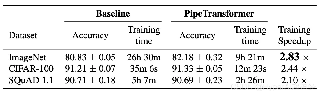
The above table summarizes the overall experimental results. Note that the speedup here is based on a conservative value a(1/3), this value can achieve similar or even higher accuracy.(2/5,1/2) can achieve higher speedup ratios, but with a slight loss in accuracy. In addition, BERT (24 layers) is larger than ViT-B/16 (12 layers), so it requires more communication time.
Performance Analysis
Speedup breakdown
This section presents the evaluation results and analyzes the performance of different components in /AutoPipe.
To understand the effectiveness of these four components and their impact on training speed, we conducted experiments with different combinations and used their training sample throughput (samples/second) and speedup as metrics. The results are shown in Figure 9.Key takeaways from the experimental results include:
1. The main speedup is the result of the elastic pipeline implemented by AutoPipe and AutoDP;
2. The effect of AutoCache is amplified by AutoDP;
3. Freeze training is conducted independently without any system adjustments or training slowdown.
Adjust a in the freezing algorithm

Figure 10: Adjusting a in the freezing algorithm
We conducted some experiments to illustrate how the freezing algorithm affects the training speed. The results show that the larger a (excessive freeze) is, the greater the speedup ratio is, but there will be a slight performance degradation. In the example shown in Figure 10, when a=1/5, frozen training is better than normal training, with a speedup ratio of 2.04.
Optimal number of chunks in an elastic pipeline

Figure 11: Optimal number of chunks in an elastic pipeline
We analyzed the optimal number of micro-batches M for different pipeline lengths K. The results are shown in Figure 11. As we can see, the optimal number M changes accordingly with different values of K. When the value of M is different, the throughput gap will also become larger (as shown in the figure when K=8), which also confirms the necessity of using anterior profiler in elastic pipelines.
Understanding Cache Timing

Figure 12: Cache timing
To evaluate AutoCache, we compared the sample throughput of training jobs starting from epoch 0 with AutoCache (blue line) and without AutoCache (red line).
Figure 12 shows that enabling caching too early slows down training because it is more expensive than a forward pass over a smaller number of frozen layers. After freezing more layers, cache activations perform significantly better than the corresponding forward pass. Therefore, AutoCache uses a Profiler to determine the right time to enable caching.
In our system, for ViT (12 layers), caching starts from the 3rd frozen layer; for BERT (24 layers), caching starts from the 5th frozen layer.
Summarize
This paper introduces PipeTransformer, a holistic solution that combines elastic pipeline parallelism and data parallelism for distributed training using the PyTorch distributed API.
Specifically, PipeTransformer can gradually freeze the layers in the pipeline, pack the remaining active layers into fewer GPUs, and fork more pipeline copies to increase the data parallel width. Evaluations on ViT and BERT models show that PipeTransformer achieves a 2.83x speedup compared to the state-of-the-art baseline without any accuracy loss.