Command Palette
Search for a command to run...
GROMACS-Tutorial Für Den Einstieg: Lysozym in Wasser
Molekulardynamik-Simulation am Beispiel „Lysozym in Wasser“
Einführung in das Tutorial
Dieses Tutorial ist ein Einführungstutorial zur Molekulardynamiksimulation mit der GROMACS-Software. Lysozym in Wasser Erfahren Sie beispielsweise, wie Sie eine molekulardynamische Simulation eines typischen Proteins in Wasser vorbereiten und ausführen.
Die GPU-Version von GROMACS mit der NVIDIA RTX 4090-Grafikkarte auf der OpenBayes-Plattform hat ihre Rechenleistung nach GPU-Parallelberechnungen mit einer Geschwindigkeit von bis zu 255 ns/Tag erheblich verbessert! Hier sind die Geschwindigkeitsleistungen:
            Core t (s)   Wall t (s)        (%)
Time:     3972.923      198.659     1999.9
                   (ns/day)    (hour/ns)
Performance:      255.471        0.094
Einführung in GROMACS
GROMACS (GROningen MAchine for Chemical Simulations) ist ein leistungsstarkes Softwarepaket für molekulardynamische Simulationen. Es wird hauptsächlich verwendet, um das Bewegungsverhalten biologischer Moleküle (wie Proteine, Lipide und Nukleinsäuren) unter verschiedenen Bedingungen zu modellieren und zu simulieren. Es wurde ursprünglich an der Universität Groningen in den Niederlanden entwickelt und hat sich zu einem der am häufigsten verwendeten Open-Source-Tools im Bereich der Molekulardynamik entwickelt.
Hauptmerkmale von GROMACS
1. hohe Leistung:
• GROMACS ist für paralleles Rechnen hochoptimiert und kann effizient auf modernen Multi-Core-CPU- und GPU-Systemen ausgeführt werden.
• Unterstützt OpenMP und MPI für Multithread- und verteiltes Computing.
2. Breites Anwendungsspektrum:
• Kann verwendet werden, um das Verhalten kleiner Moleküle gegenüber großen Proteinkomplexen zu simulieren.
• Unterstützt die Forschung zu Biomolekülen, Polymeren, anorganischen Verbindungen und anderen chemischen Systemen.
3. Flexibilität:
• Bietet eine Vielzahl von Tools für die Vorverarbeitung (z. B. Topologiegenerierung, Solvatation) und Nachverarbeitung (z. B. Trajektorienanalyse, Energieberechnung).
• Unterstützung für verschiedene Kraftfelder wie AMBER, CHARMM und GROMOS.
4. Benutzerfreundlichkeit:
• GROMACS enthält eine benutzerfreundliche Befehlszeilenschnittstelle.
• Bietet ausführliche Dokumentationen und Tutorials, die sowohl für Anfänger als auch für fortgeschrittene Benutzer geeignet sind.
5. Open Source und skalierbar:
• Die Open-Source-Lizenz ermöglicht es Benutzern, GROMACS an spezifische Anforderungen anzupassen und zu erweitern.
• Verfügt über eine aktive Benutzer-Community und ein Entwicklungsteam.
Allgemeiner Nutzungsprozess von GROMACS
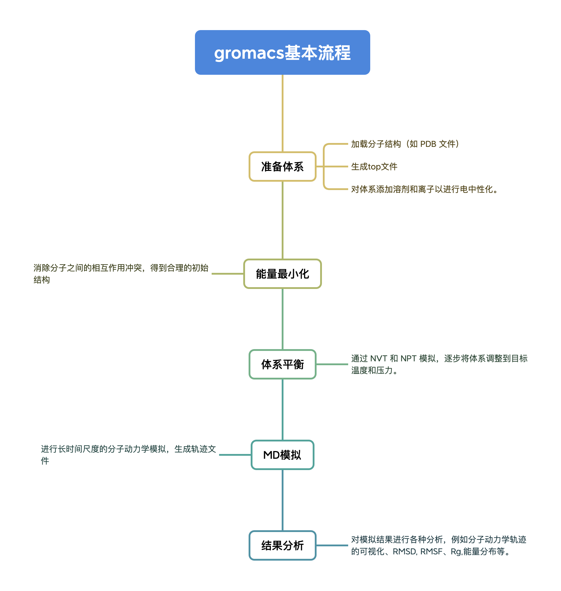
Schritte ausführen
Zuerst müssen wir die PDB-Proteindatei und die MD-Berechnungsdatei konfigurieren. Nach verschiedenen Vorverarbeitungen führen wir schließlich eine 10-ns-Simulation durch und analysieren die Ergebnisse. Nachfolgend finden Sie eine schrittweise Erklärung.
1. Starten Sie GROMACS
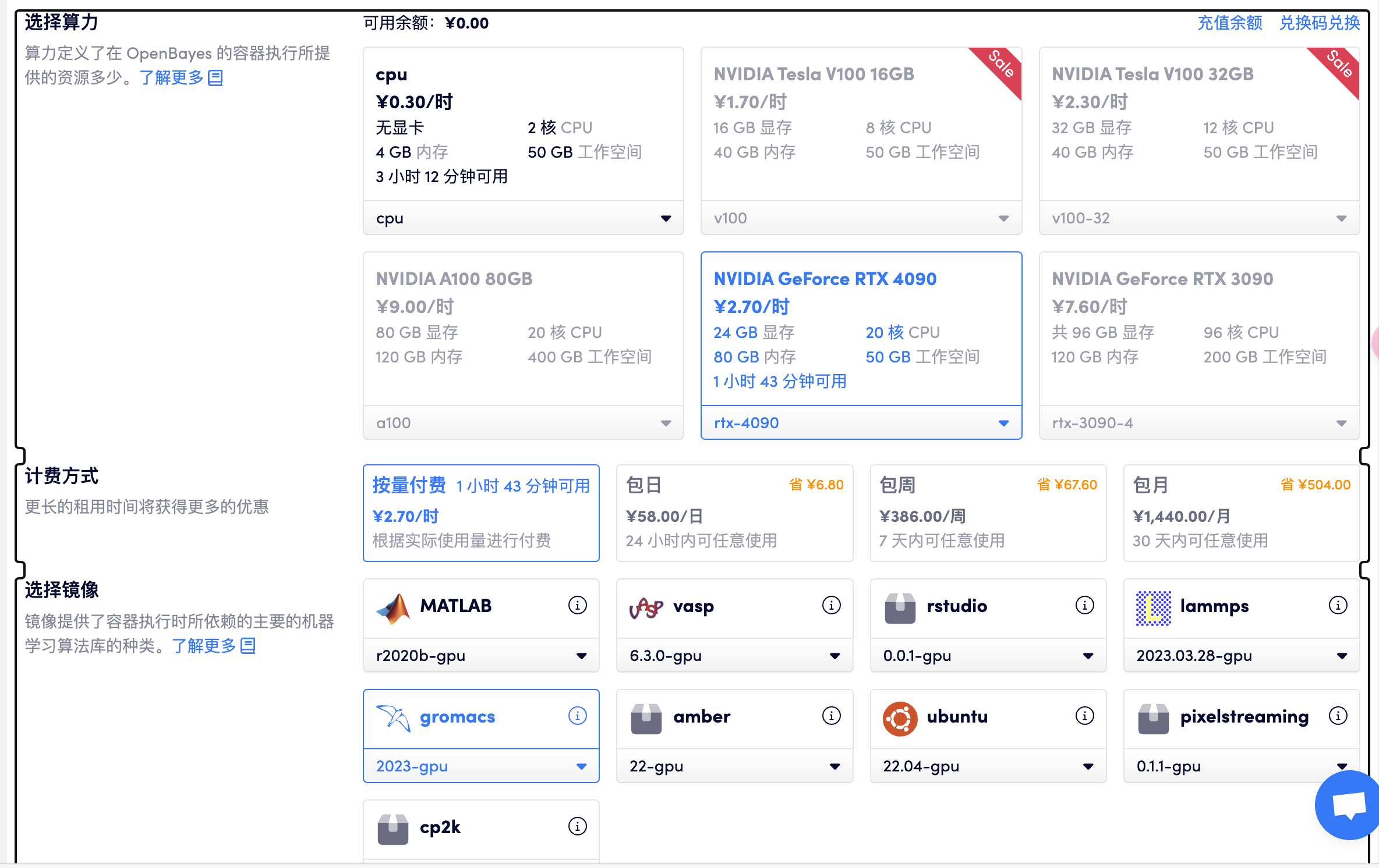
首先登录平台:https://openbayes.com/

选择「高性能计算」> 创建新容器> 选择算力 RTX 4090> 选择 gromacs GPU
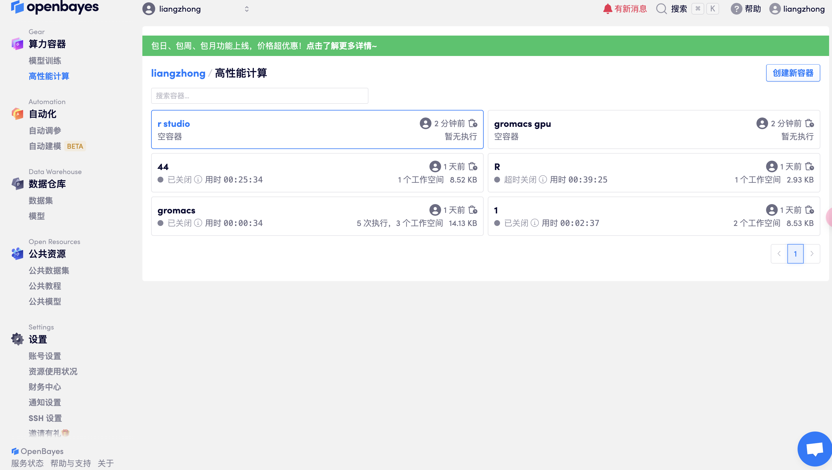

打开工作空间

打开终端

或者采用 SSH 控制服务器:

在 X-shell 或者 mac unix 终端,输入:ssh -p 32699  [email protected],再输入密码即可(如下所示)↓
liangzhongzhongzhong@lzr ~ % ssh -p 32699  [email protected]
The authenticity of host '[ssh.openbayes.com]:32699 ([101.237.34.75]:32699)' can't be established.
ED25519 key fingerprint is SHA256:uwPyhP/EYoW49Ez4rvAuaf19czwis2rdS4pImsR0NH8.
This key is not known by any other names.
Are you sure you want to continue connecting (yes/no/[fingerprint])? yes
Warning: Permanently added '[ssh.openbayes.com]:32699' (ED25519) to the list of known hosts.
[email protected]'s password:
OpenBayes

目录说明

- /openbayes/home 工作空间内的数据保存地址,容器停止后,该目录中的内容不会被删除
- /openbayes/input/input0 - /openbayes/input/input4 为数据目录,不会占用工作空间的存储容量,最多支持同时绑定 5 个

⚠️  其他目录下的内容在容器关闭后会被自动删除!更多信息请访问 https://openbayes.com/docs/concepts
⚠️  禁止挖矿,一经发现将立即封号恕不退款

(base) root@liangzhong-4ay9ej85pxvd-main:/openbayes/home# ls
(base) root@liangzhong-4ay9ej85pxvd-main:/openbayes# l(base) root@liangzhong-4ay9ej85pxvd-main:/openbayes# lhome  input  请将文件存在 home 目录下, 当前文件夹下的文件不会被保存.txt
(base) root@liangzhong-4ay9ej85pxvd-main:/openbayes# ls(base) root@liangzhong-4ay9ej85pxvd-main:/openbaye
(base) root@liangzhong-4ay9ej85pxvd-main:/openbayes/input# cd input0
(base) root@liangzhong-4ay9ej85pxvd-main:/openbayes/input/input0# ls
'#nvt.log.1#'    '#topol.top.2#'    1AKI_processed.gro   1aki.pdb   em.log   ions.mdp   mdout.mdp   nvt.cpt   nvt.log   nvt.trr         topol.top
'#nvt.log.2#'     1AKI_clean.pdb    1AKI_solv.gro        em.edr     em.tpr   ions.tpr   minim.mdp   nvt.edr   nvt.mdp   posre.itp
'#topol.top.1#'   1AKI_newbox.gro   1AKI_solv_ions.gro   em.gro     em.trr   md.mdp     npt.mdp     nvt.gro   nvt.tpr   potential.xvg
(base) root@liangzhong-4ay9ej85pxvd-main:/openbayes/input/input0#

调用 GROMACS,设置临时环境变量
export PATH=/data/app/gromacs/bin:$PATH
(base) root@liangzhong-4ay9ej85pxvd-main:/openbayes/home# gmx_mpi -h
                        :-) GROMACS - gmx_mpi, 2023 (-:

Executable:   /data/app/gromacs/bin/gmx_mpi
Data prefix:  /data/app/gromacs
Working dir:  /output
Command line:
  gmx_mpi -h

SYNOPSIS

gmx [-[no]h] [-[no]quiet] [-[no]version] [-[no]copyright] [-nice <int>]
    [-[no]backup]

OPTIONS

Other options:

 -[no]h                     (no)
           Print help and quit
 -[no]quiet                 (no)
           Do not print common startup info or quotes
 -[no]version               (no)
           Print extended version information and quit
 -[no]copyright             (no)
           Print copyright information on startup
 -nice   <int>              (19)
           Set the nicelevel (default depends on command)
 -[no]backup                (yes)
           Write backups if output files exist

Additional help is available on the following topics:
    commands    List of available commands
    selections  Selection syntax and usage
To access the help, use 'gmx help <topic>'.
For help on a command, use 'gmx help <command>'.

GROMACS reminds you: "All You Need is Greed" (Aztec Camera)
2. Dokumentenvorbereitung
Bevor wir das Tutorial ausführen, müssen wir die folgenden 6 Dateien vorbereiten: 1aki.pdb, ions.mdp, md.mdp, minim.mdp, npt.mdp, nvt.mdp
Diese Dateien können direkt heruntergeladen oder wie folgt erstellt werden.
Beispielsweise kann die Proteindatei 1AKI.pdb von RCSB Holen Sie sich 1AKI.pdb von der Website.Im Tutorial wurden andere Dateien erstellt, indem der Code mit dem Vim-Texteditor kopiert wurde.
Einführung in die RCSB-Datenbank:
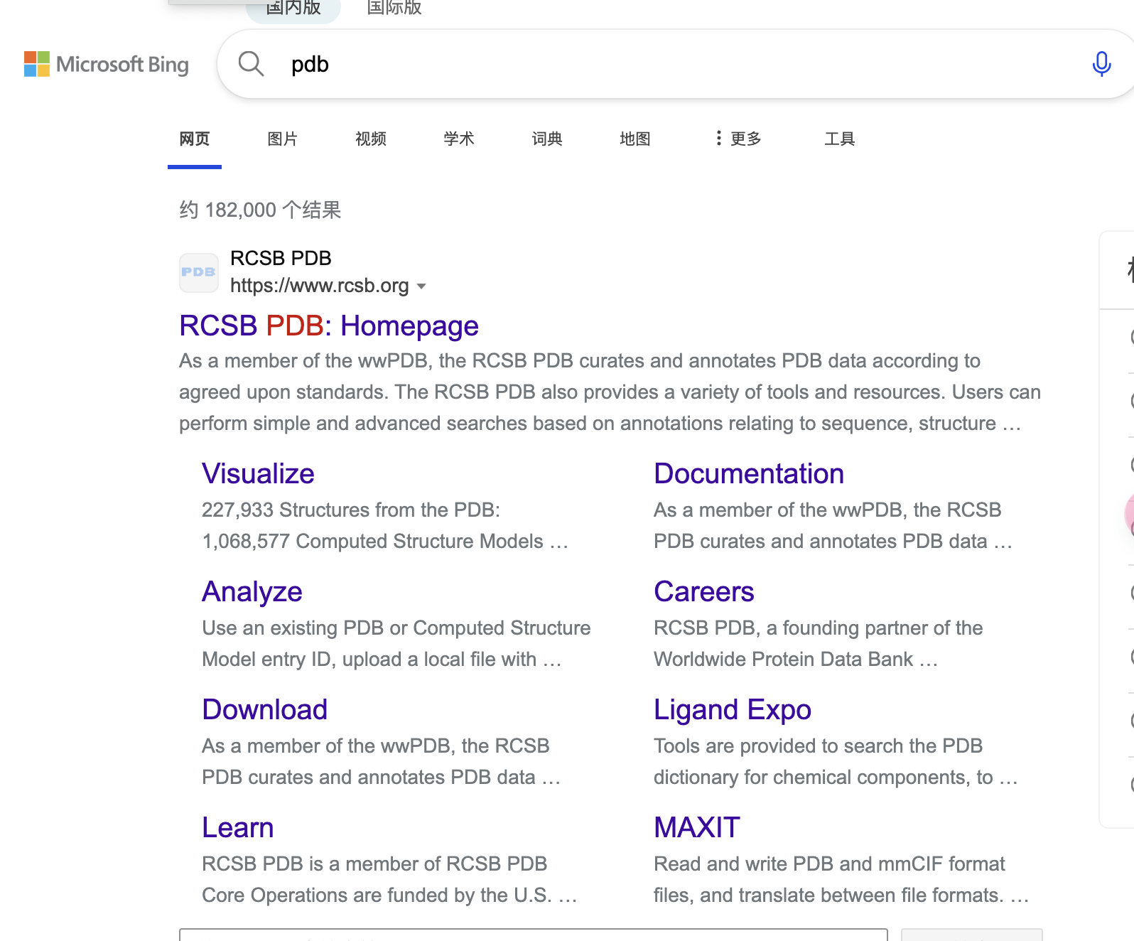
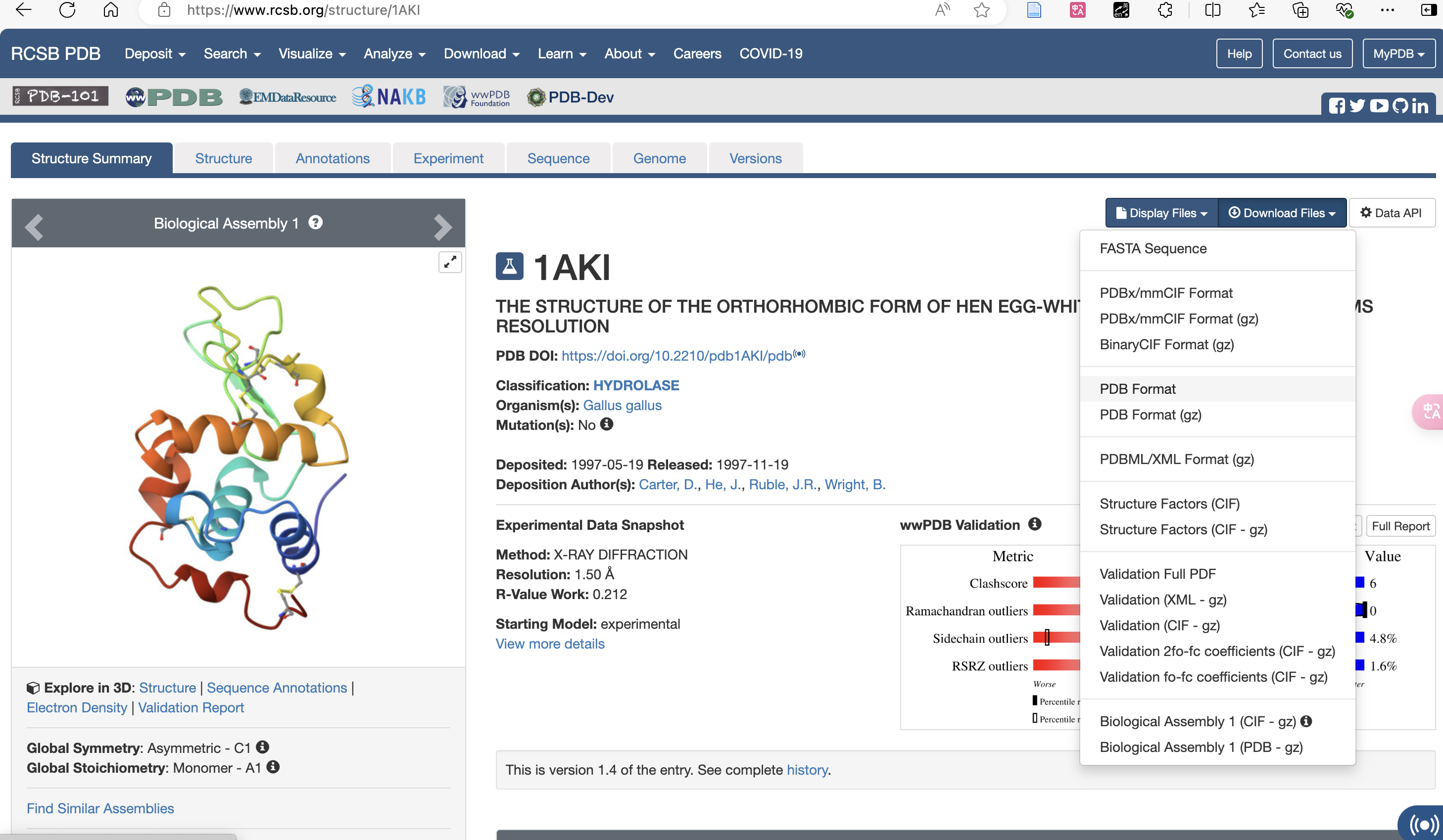
PDF-Format herunterladen:
In Ihr Arbeitsverzeichnis hochladen
(base) root@liangzhong-4ay9ej85pxvd-main:/input0# ls
1aki.pdb
#查看上传成功
vim ions.mdp
#准备 mdp 文件,输入命令后复制一下内容,按 i 进入插入模式开始编辑。
#编辑完成后,按 Esc 键退出插入模式,输入 :wq 保存并退出。
; ions.mdp - used as input into grompp to generate ions.tpr
; Parameters describing what to do, when to stop and what to save
integrator  = steep         ; Algorithm (steep = steepest descent minimization)
emtol       = 1000.0        ; Stop minimization when the maximum force < 1000.0 kJ/mol/nm
emstep      = 0.01          ; Minimization step size
nsteps      = 50000         ; Maximum number of (minimization) steps to perform

; Parameters describing how to find the neighbors of each atom and how to calculate the interactions
nstlist         = 1         ; Frequency to update the neighbor list and long range forces
cutoff-scheme	= Verlet    ; Buffered neighbor searching
ns_type         = grid      ; Method to determine neighbor list (simple, grid)
coulombtype     = cutoff    ; Treatment of long range electrostatic interactions
rcoulomb        = 1.0       ; Short-range electrostatic cut-off
rvdw            = 1.0       ; Short-range Van der Waals cut-off
pbc             = xyz       ; Periodic Boundary Conditions in all 3 dimensions
vim minim.mdp

; minim.mdp - used as input into grompp to generate em.tpr
; Parameters describing what to do, when to stop and what to save
integrator  = steep         ; Algorithm (steep = steepest descent minimization)
emtol       = 1000.0        ; Stop minimization when the maximum force < 1000.0 kJ/mol/nm
emstep      = 0.01          ; Minimization step size
nsteps      = 50000         ; Maximum number of (minimization) steps to perform

; Parameters describing how to find the neighbors of each atom and how to calculate the interactions
nstlist         = 1         ; Frequency to update the neighbor list and long range forces
cutoff-scheme   = Verlet    ; Buffered neighbor searching
ns_type         = grid      ; Method to determine neighbor list (simple, grid)
coulombtype     = PME       ; Treatment of long range electrostatic interactions
rcoulomb        = 1.0       ; Short-range electrostatic cut-off
rvdw            = 1.0       ; Short-range Van der Waals cut-off
pbc             = xyz       ; Periodic Boundary Conditions in all 3 dimensions
vim nvt.mdp

title                   = OPLS Lysozyme NVT equilibration
define                  = -DPOSRES  ; position restrain the protein
; Run parameters
integrator              = md        ; leap-frog integrator
nsteps                  = 50000     ; 2 * 50000 = 100 ps
dt                      = 0.002     ; 2 fs
; Output control
nstxout                 = 500       ; save coordinates every 1.0 ps
nstvout                 = 500       ; save velocities every 1.0 ps
nstenergy               = 500       ; save energies every 1.0 ps
nstlog                  = 500       ; update log file every 1.0 ps
; Bond parameters
continuation            = no        ; first dynamics run
constraint_algorithm    = lincs     ; holonomic constraints
constraints             = h-bonds   ; bonds involving H are constrained
lincs_iter              = 1         ; accuracy of LINCS
lincs_order             = 4         ; also related to accuracy
; Nonbonded settings
cutoff-scheme           = Verlet    ; Buffered neighbor searching
ns_type                 = grid      ; search neighboring grid cells
nstlist                 = 10        ; 20 fs, largely irrelevant with Verlet
rcoulomb                = 1.0       ; short-range electrostatic cutoff (in nm)
rvdw                    = 1.0       ; short-range van der Waals cutoff (in nm)
DispCorr                = EnerPres  ; account for cut-off vdW scheme
; Electrostatics
coulombtype             = PME       ; Particle Mesh Ewald for long-range electrostatics
pme_order               = 4         ; cubic interpolation
fourierspacing          = 0.16      ; grid spacing for FFT
; Temperature coupling is on
tcoupl                  = V-rescale             ; modified Berendsen thermostat
tc-grps                 = Protein Non-Protein   ; two coupling groups - more accurate
tau_t                   = 0.1     0.1           ; time constant, in ps
ref_t                   = 300     300           ; reference temperature, one for each group, in K
; Pressure coupling is off
pcoupl                  = no        ; no pressure coupling in NVT
; Periodic boundary conditions
pbc                     = xyz       ; 3-D PBC
; Velocity generation
gen_vel                 = yes       ; assign velocities from Maxwell distribution
gen_temp                = 300       ; temperature for Maxwell distribution
gen_seed                = -1        ; generate a random seed
vim npt.mdp

title                   = OPLS Lysozyme NPT equilibration
define                  = -DPOSRES  ; position restrain the protein
; Run parameters
integrator              = md        ; leap-frog integrator
nsteps                  = 50000     ; 2 * 50000 = 100 ps
dt                      = 0.002     ; 2 fs
; Output control
nstxout                 = 500       ; save coordinates every 1.0 ps
nstvout                 = 500       ; save velocities every 1.0 ps
nstenergy               = 500       ; save energies every 1.0 ps
nstlog                  = 500       ; update log file every 1.0 ps
; Bond parameters
continuation            = yes       ; Restarting after NVT
constraint_algorithm    = lincs     ; holonomic constraints
constraints             = h-bonds   ; bonds involving H are constrained
lincs_iter              = 1         ; accuracy of LINCS
lincs_order             = 4         ; also related to accuracy
; Nonbonded settings
cutoff-scheme           = Verlet    ; Buffered neighbor searching
ns_type                 = grid      ; search neighboring grid cells
nstlist                 = 10        ; 20 fs, largely irrelevant with Verlet scheme
rcoulomb                = 1.0       ; short-range electrostatic cutoff (in nm)
rvdw                    = 1.0       ; short-range van der Waals cutoff (in nm)
DispCorr                = EnerPres  ; account for cut-off vdW scheme
; Electrostatics
coulombtype             = PME       ; Particle Mesh Ewald for long-range electrostatics
pme_order               = 4         ; cubic interpolation
fourierspacing          = 0.16      ; grid spacing for FFT
; Temperature coupling is on
tcoupl                  = V-rescale             ; modified Berendsen thermostat
tc-grps                 = Protein Non-Protein   ; two coupling groups - more accurate
tau_t                   = 0.1     0.1           ; time constant, in ps
ref_t                   = 300     300           ; reference temperature, one for each group, in K
; Pressure coupling is on
pcoupl                  = Parrinello-Rahman     ; Pressure coupling on in NPT
pcoupltype              = isotropic             ; uniform scaling of box vectors
tau_p                   = 2.0                   ; time constant, in ps
ref_p                   = 1.0                   ; reference pressure, in bar
compressibility         = 4.5e-5                ; isothermal compressibility of water, bar^-1
refcoord_scaling        = com
; Periodic boundary conditions
pbc                     = xyz       ; 3-D PBC
; Velocity generation
gen_vel                 = no        ; Velocity generation is off
vim md.md

title                   = OPLS Lysozyme NPT equilibration
; Run parameters
integrator              = md        ; leap-frog integrator
nsteps                  = 500000    ; 2 * 500000 = 1000 ps (1 ns)
dt                      = 0.002     ; 2 fs
; Output control
nstxout                 = 0         ; suppress bulky .trr file by specifying
nstvout                 = 0         ; 0 for output frequency of nstxout,
nstfout                 = 0         ; nstvout, and nstfout
nstenergy               = 5000      ; save energies every 10.0 ps
nstlog                  = 5000      ; update log file every 10.0 ps
nstxout-compressed      = 5000      ; save compressed coordinates every 10.0 ps
compressed-x-grps       = System    ; save the whole system
; Bond parameters
continuation            = yes       ; Restarting after NPT
constraint_algorithm    = lincs     ; holonomic constraints
constraints             = h-bonds   ; bonds involving H are constrained
lincs_iter              = 1         ; accuracy of LINCS
lincs_order             = 4         ; also related to accuracy
; Neighborsearching
cutoff-scheme           = Verlet    ; Buffered neighbor searching
ns_type                 = grid      ; search neighboring grid cells
nstlist                 = 10        ; 20 fs, largely irrelevant with Verlet scheme
rcoulomb                = 1.0       ; short-range electrostatic cutoff (in nm)
rvdw                    = 1.0       ; short-range van der Waals cutoff (in nm)
; Electrostatics
coulombtype             = PME       ; Particle Mesh Ewald for long-range electrostatics
pme_order               = 4         ; cubic interpolation
fourierspacing          = 0.16      ; grid spacing for FFT
; Temperature coupling is on
tcoupl                  = V-rescale             ; modified Berendsen thermostat
tc-grps                 = Protein Non-Protein   ; two coupling groups - more accurate
tau_t                   = 0.1     0.1           ; time constant, in ps
ref_t                   = 300     300           ; reference temperature, one for each group, in K
; Pressure coupling is on
pcoupl                  = Parrinello-Rahman     ; Pressure coupling on in NPT
pcoupltype              = isotropic             ; uniform scaling of box vectors
tau_p                   = 2.0                   ; time constant, in ps
ref_p                   = 1.0                   ; reference pressure, in bar
compressibility         = 4.5e-5                ; isothermal compressibility of water, bar^-1
; Periodic boundary conditions
pbc                     = xyz       ; 3-D PBC
; Dispersion correction
DispCorr                = EnerPres  ; account for cut-off vdW scheme
; Velocity generation
gen_vel                 = no        ; Velocity generation is off
2. Formale Simulationsschritte
Ziel: Erstellen Sie ein physikalisch sinnvolles Simulationssystem, um die Grundlage für die nachfolgende dynamische Simulation zu legen.
1. Molekularstruktur laden (PDB-Datei):
• PDB-Dateien(Protein Data Bank) enthält dreidimensionale Koordinaten und Strukturinformationen von Molekülen (wie Proteinen, Nukleinsäuren und kleinen Molekülen).
• GROMACS verwendet das Tool pdb2gmx, um diese Koordinateninformationen in ein Molekülmodell umzuwandeln und Kraftfeldparameter zuzuweisen.
• Kraftfeld: Ein mathematisches Modell, das die Wechselwirkungen zwischen Molekülen beschreibt, einschließlich Bindungen, Winkeln, Diederpotentialenergie, Van-der-Waals-Kräften und Ladungswechselwirkungen.
• Gemeinsame Kraftfelder: GROMOS, AMBER, CHARMM.
(Häufig verwendete sind AMBER99SB-Protein, OPLS-AA/L-Allatom-Kraftfeld, Charm36-Kraftfeld (müssen selbst heruntergeladen und konfiguriert werden), andere Kraftfelder sind zu alt und nicht zum Veröffentlichen von Artikeln geeignet)
2. Topologiedatei generieren:
• Die Topologiedatei (topol.top) definiert die Kraftfeldparameter jedes Moleküls im Simulationssystem, wie etwa Atomtyp, Bindungstyp und dessen Parameter usw.
• Es bildet in Kombination mit der Koordinatendatei die Grundlage für molekulardynamische Simulationen.
3. Führen Sie pdb2gmx aus, wählen Sie Kraftfeld: 15 und drücken Sie die Eingabetaste
#删除水分子(PDB 文件中的 “HOH” 残基)
grep -v HOH 1aki.pdb > 1AKI_clean.pdb
gmx_mpi pdb2gmx -f 1AKI_clean.pdb -o 1AKI_processed.gro -water spce
#选择 15,按回车,OPLS-AA/L all-atom force field (2001 aminoacid dihedrals)

(base) root@liangzhong-4ay9ej85pxvd-main:/input0#  pdb2gmx -f 1AKI_clean.pdb -o 1AKI_processed.gro -water spce
                      :-) GROMACS - gmx pdb2gmx, 2023 (-:

Executable:   /data/app/gromacs/bin/gmx_mpi
Data prefix:  /data/app/gromacs
Working dir:  /input0
Command line:
  gmx_mpi pdb2gmx -f 1AKI_clean.pdb -o 1AKI_processed.gro -water spce

Select the Force Field:

From '/data/app/gromacs/share/gromacs/top':

 1: AMBER03 protein, nucleic AMBER94 (Duan et al., J. Comp. Chem. 24, 1999-2012, 2003)

 2: AMBER94 force field (Cornell et al., JACS 117, 5179-5197, 1995)

 3: AMBER96 protein, nucleic AMBER94 (Kollman et al., Acc. Chem. Res. 29, 461-469, 1996)

 4: AMBER99 protein, nucleic AMBER94 (Wang et al., J. Comp. Chem. 21, 1049-1074, 2000)

 5: AMBER99SB protein, nucleic AMBER94 (Hornak et al., Proteins 65, 712-725, 2006)

 6: AMBER99SB-ILDN protein, nucleic AMBER94 (Lindorff-Larsen et al., Proteins 78, 1950-58, 2010)

 7: AMBERGS force field (Garcia & Sanbonmatsu, PNAS 99, 2782-2787, 2002)

 8: CHARMM27 all-atom force field (CHARM22 plus CMAP for proteins)

 9: GROMOS96 43a1 force field

10: GROMOS96 43a2 force field (improved alkane dihedrals)

11: GROMOS96 45a3 force field (Schuler JCC 2001 22 1205)

12: GROMOS96 53a5 force field (JCC 2004 vol 25 pag 1656)

13: GROMOS96 53a6 force field (JCC 2004 vol 25 pag 1656)

14: GROMOS96 54a7 force field (Eur. Biophys. J. (2011), 40,, 843-856, DOI: 10.1007/s00249-011-0700-9)

15: OPLS-AA/L all-atom force field (2001 aminoacid dihedrals)
15

Using the Oplsaa force field in directory oplsaa.ff

going to rename oplsaa.ff/aminoacids.r2b
Opening force field file /data/app/gromacs/share/gromacs/top/oplsaa.ff/aminoacids.r2b
Reading 1AKI_clean.pdb...
WARNING: all CONECT records are ignored
Read 'LYSOZYME', 1001 atoms

Analyzing pdb file
Splitting chemical chains based on TER records or chain id changing.

There are 1 chains and 0 blocks of water and 129 residues with 1001 atoms

  chain  #res #atoms

  1 'A'   129   1001

All occupancies are one
All occupancies are one
Opening force field file /data/app/gromacs/share/gromacs/top/oplsaa.ff/atomtypes.atp

Reading residue database... (Oplsaa)
Opening force field file /data/app/gromacs/share/gromacs/top/oplsaa.ff/aminoacids.rtp
Opening force field file /data/app/gromacs/share/gromacs/top/oplsaa.ff/aminoacids.hdb
Opening force field file /data/app/gromacs/share/gromacs/top/oplsaa.ff/aminoacids.n.tdb
Opening force field file /data/app/gromacs/share/gromacs/top/oplsaa.ff/aminoacids.c.tdb

Processing chain 1 'A' (1001 atoms, 129 residues)
Analysing hydrogen-bonding network for automated assignment of histidine
 protonation. 213 donors and 184 acceptors were found.
There are 255 hydrogen bonds
Will use HISE for residue 15

Identified residue LYS1 as a starting terminus.

Identified residue LEU129 as a ending terminus.
8 out of 8 lines of specbond.dat converted successfully
Special Atom Distance matrix:
                    CYS6   MET12   HIS15   CYS30   CYS64   CYS76   CYS80
                    SG48    SD87  NE2118   SG238   SG513   SG601   SG630
   MET12    SD87   1.166
   HIS15  NE2118   1.776   1.019
   CYS30   SG238   1.406   1.054   2.069
   CYS64   SG513   2.835   1.794   1.789   2.241
   CYS76   SG601   2.704   1.551   1.468   2.116   0.765
   CYS80   SG630   2.959   1.951   1.916   2.391   0.199   0.944
   CYS94   SG724   2.550   1.407   1.382   1.975   0.665   0.202   0.855
  MET105   SD799   1.827   0.911   1.683   0.888   1.849   1.461   2.036
  CYS115   SG889   1.576   1.084   2.078   0.200   2.111   1.989   2.262
  CYS127   SG981   0.197   1.072   1.721   1.313   2.799   2.622   2.934
                   CYS94  MET105  CYS115
                   SG724   SD799   SG889
  MET105   SD799   1.381
  CYS115   SG889   1.853   0.790
  CYS127   SG981   2.475   1.686   1.483
Linking CYS-6 SG-48 and CYS-127 SG-981...
Linking CYS-30 SG-238 and CYS-115 SG-889...
Linking CYS-64 SG-513 and CYS-80 SG-630...
Linking CYS-76 SG-601 and CYS-94 SG-724...
Start terminus LYS-1: NH3+
End terminus LEU-129: COO-

Checking for duplicate atoms....

Generating any missing hydrogen atoms and/or adding termini.

Now there are 129 residues with 1960 atoms

Making bonds...

Number of bonds was 1984, now 1984

Generating angles, dihedrals and pairs...
Before cleaning: 5142 pairs
Before cleaning: 5187 dihedrals

Making cmap torsions...

There are 5187 dihedrals,  426 impropers, 3547 angles
          5106 pairs,     1984 bonds and     0 virtual sites

Total mass 14313.193 a.m.u.

Total charge 8.000 e

Writing topology

Writing coordinate file...

                --------- PLEASE NOTE ------------

You have successfully generated a topology from: 1AKI_clean.pdb.

The Oplsaa force field and the spce water model are used.

                --------- ETON ESAELP ------------

GROMACS reminds you: "Any one who considers arithmetical methods of producing random digits is, of course, in a state of sin." (John von Neumann)
Sie können sehen, dass es mehrere weitere Dateien gibt, und "Gesamtgebühr 8.000 e" Wir müssen die Gebühr später neutralisieren
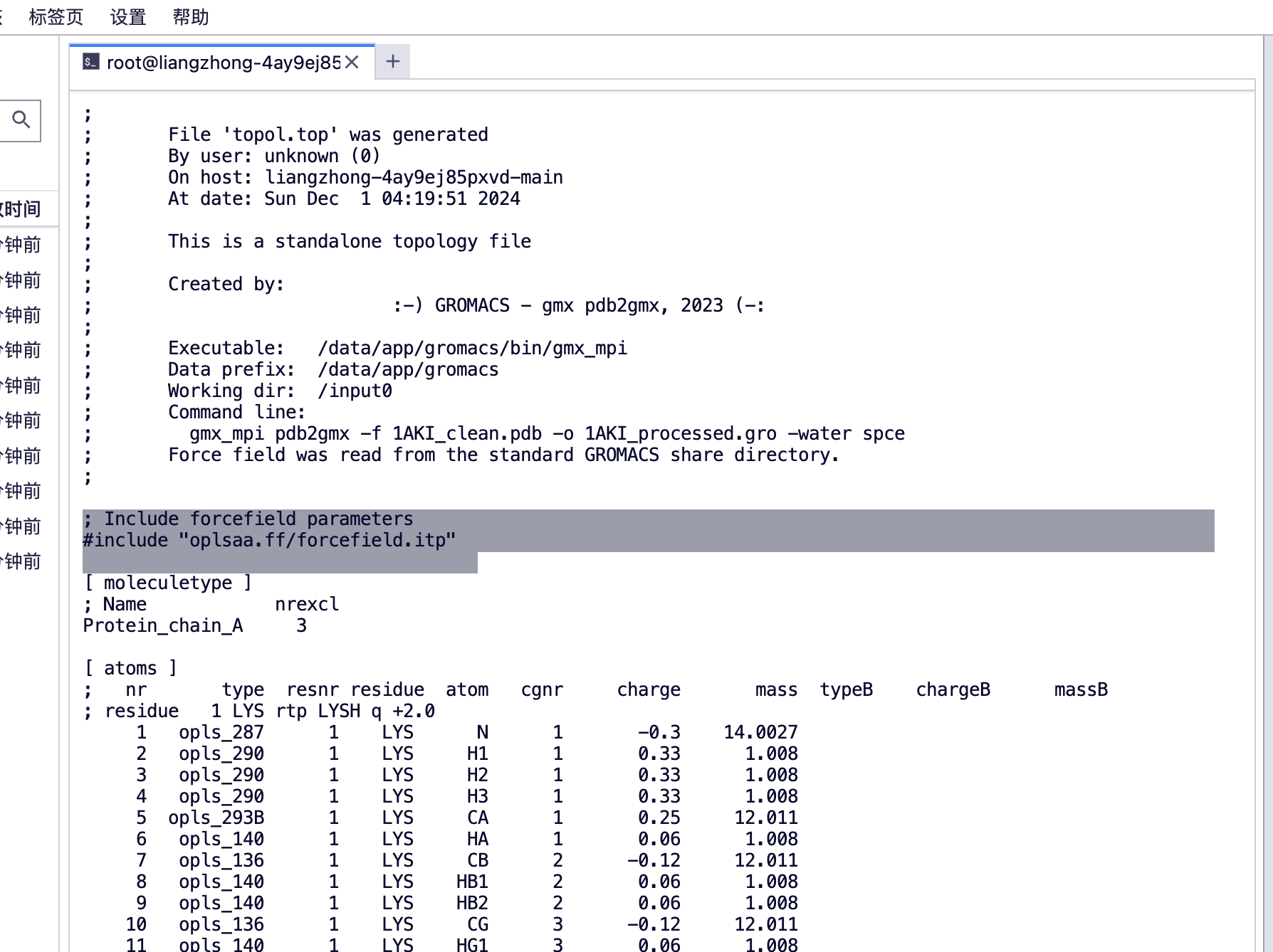
Verwenden Sie den Vim-Befehl, um topol.top anzuzeigen, und Sie können das Kraftfeld-Tag sehen.
(base) root@liangzhong-4ay9ej85pxvd-main:/input0# ls
1AKI_clean.pdb      1aki.pdb  md.mdp     npt.mdp  posre.itp
1AKI_processed.gro  ions.mdp  minim.mdp  nvt.mdp  topol.top
4. Erstellen Sie eine rhombische Dodekaeder-Box, um das Protein einzuschließen, damit wir Lösungsmittelmoleküle hinzufügen können
• Auswahl der Kastenform: Zu den gängigen Formen von Simulationsboxen zählen Würfel, orthogonale Boxen, Rhombendodekaeder usw. Normalerweise werden Formen gewählt, mit denen Moleküle effektiv gefüllt werden können und die den Rechenaufwand reduzieren.
gmx_mpi editconf -f 1AKI_processed.gro -o 1AKI_newbox.gro -c -d 1.0 -bt cubic

#将蛋白质在框中居中(-c),并将其放置在框边缘至少 1.0 nm 的位置(-d 1.0)

Command line:
  gmx_mpi editconf -f 1AKI_processed.gro -o 1AKI_newbox.gro -c -d 1.0 -bt cubic

Note that major changes are planned in future for editconf, to improve usability and utility.
Read 1960 atoms
Volume: 123.376 nm^3, corresponds to roughly 55500 electrons
No velocities found
    system size :  3.817  4.234  3.454 (nm)
    diameter    :  5.010               (nm)
    center      :  2.781  2.488  0.017 (nm)
    box vectors :  5.906  6.845  3.052 (nm)
    box angles  :  90.00  90.00  90.00 (degrees)
    box volume  : 123.38               (nm^3)
    shift       :  0.724  1.017  3.488 (nm)
new center      :  3.505  3.505  3.505 (nm)
new box vectors :  7.010  7.010  7.010 (nm)
new box angles  :  90.00  90.00  90.00 (degrees)
new box volume  : 344.48               (nm^3)
5. Definieren Sie eine Box und fügen Sie Lösungsmittel (Wasser) hinzu
Zweck:Lösung: Platzieren Sie Moleküle in einer Lösungsmittelumgebung (z. B. einer Wasserbox), um ihr Verhalten in der realen Umgebung zu simulieren.
gmx_mpi solvate -cp 1AKI_newbox.gro -cs spc216.gro -o 1AKI_solv.gro -p topol.top

#结果
Generating solvent configuration
Will generate new solvent configuration of 4x4x4 boxes
Solvent box contains 39252 atoms in 13084 residues
Removed 5451 solvent atoms due to solvent-solvent overlap
Removed 1869 solvent atoms due to solute-solvent overlap
Sorting configuration
Found 1 molecule type:
    SOL (   3 atoms): 10644 residues
Generated solvent containing 31932 atoms in 10644 residues
Writing generated configuration to 1AKI_solv.gro

Output configuration contains 33892 atoms in 10773 residues
Volume                 :     344.484 (nm^3)
Density                :     997.935 (g/l)
Number of solvent molecules:  10644

Processing topology
Adding line for 10644 solvent molecules with resname (SOL) to topology file (topol.top)

#查看一下 top 文件
(base) root@liangzhong-4ay9ej85pxvd-main:/input0# ls
'#topol.top.1#'   1AKI_newbox.gro      1AKI_solv.gro   ions.mdp   minim.mdp   nvt.mdp     topol.top
 1AKI_clean.pdb   1AKI_processed.gro   1aki.pdb        md.mdp     npt.mdp     posre.itp
(base) root@liangzhong-4ay9ej85pxvd-main:/input0# vim topol.top
#查看 top 文件的末尾
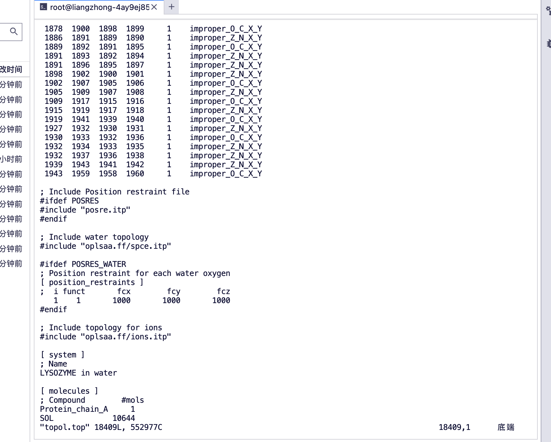
Sie können [Moleküle] sehen
protein_chain_A, Protein-A-Kette
SOL Wassermolekül
6. Assemblieren Sie die .tpr-Datei
gmx_mpi grompp -f ions.mdp -c 1AKI_solv.gro -p topol.top -o ions.tpr
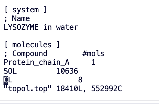
7. Neutralisieren Sie die Ladung und ersetzen Sie die Lösungsmittelmoleküle durch Ionen
Ladungsneutralisierung:Fügen Sie Ionen (wie Na⁺, Cl⁻) hinzu, um die Gesamtladung des Systems zu neutralisieren und Simulationsverzerrungen durch elektrostatische Effekte zu vermeiden.
gmx_mpi genion -s ions.tpr -o 1AKI_solv_ions.gro -p topol.top -pname NA -nname CL -neutral
Command line:
  gmx_mpi genion -s ions.tpr -o 1AKI_solv_ions.gro -p topol.top -pname NA -nname CL -neutral

Reading file ions.tpr, VERSION 2023 (single precision)
Reading file ions.tpr, VERSION 2023 (single precision)
Will try to add 0 NA ions and 8 CL ions.
Select a continuous group of solvent molecules
Group     0 (         System) has 33892 elements
Group     1 (        Protein) has  1960 elements
Group     2 (      Protein-H) has  1001 elements
Group     3 (        C-alpha) has   129 elements
Group     4 (       Backbone) has   387 elements
Group     5 (      MainChain) has   517 elements
Group     6 (   MainChain+Cb) has   634 elements
Group     7 (    MainChain+H) has   646 elements
Group     8 (      SideChain) has  1314 elements
Group     9 (    SideChain-H) has   484 elements
Group    10 (    Prot-Masses) has  1960 elements
Group    11 (    non-Protein) has 31932 elements
Group    12 (          Water) has 31932 elements
Group    13 (            SOL) has 31932 elements
Group    14 (      non-Water) has  1960 elements
Select a group: 13
Selected 13: 'SOL'
Number of (3-atomic) solvent molecules: 10644

Processing topology
Replacing 8 solute molecules in topology file (topol.top)  by 0 NA and 8 CL ions.

Back Off! I just backed up topol.top to ./#topol.top.2#
Using random seed -1212354563.
Replacing solvent molecule 3671 (atom 12973) with CL
Replacing solvent molecule 2264 (atom 8752) with CL
Replacing solvent molecule 2559 (atom 9637) with CL
Replacing solvent molecule 8081 (atom 26203) with CL
Replacing solvent molecule 8468 (atom 27364) with CL
Replacing solvent molecule 7439 (atom 24277) with CL
Replacing solvent molecule 9983 (atom 31909) with CL
Replacing solvent molecule 650 (atom 3910) with CL

GROMACS reminds you: "Water is just water" (Berk Hess)

(base) root@liangzhong-4ay9ej85pxvd-main:/input0#
Man sieht, dass viele Chloridionen hinzugefügt wurden
8. Energieminimierung
8.1 Grund: Wenn wir eine molekulardynamische Simulation durchführen, werden die von uns erhaltenen pdb-Dateien durch Röntgen-, Elektronenmikroskopie und andere Methoden gewonnen, die viele Bindungswinkel und Verzerrungen mit übermäßiger Energie oder die Bildung oder das Aufbrechen von Wasserstoffbrücken, spezielle Anordnungen zwischen Molekülen und hohe Energie aufgrund des geringen Abstands zwischen Atomen enthalten, was es für das molekulare System in der Simulation schwierig macht, von einem energiereichen Zustand in einen energiearmen Zustand überzugehen. Diese Methode ist erforderlich, um die Energie des Systems zu minimieren.
8.2 Prinzip: Das Grundprinzip der Energieminimierung: Die Energieminimierung basiert auf der potentiellen Energiefunktion, die die gesamte potentielle Energie des Systems durch iterative Berechnung und Anpassung der Atomkoordinaten reduziert. Zu den häufig verwendeten Methoden gehören:
① Konjugierte Gradientenmethode: Eine Gradientenabstiegsmethode, die die Konvergenz durch Nutzung von Informationen aus dem vorherigen Schritt beschleunigt.
② Methode des steilsten Abstiegs: Jede Iteration bewegt sich in die entgegengesetzte Richtung des potenziellen Energiegradienten und reduziert die Energie über den steilsten Abstiegspfad.
3. Newton-Raphson-Methode: Eine Methode der Ableitung zweiter Ordnung, die die Ableitung zweiter Ordnung der potentiellen Energiefunktion verwendet, um den Punkt minimaler Energie genauer zu finden.
8.3 Zweck: Finden einer stabileren Molekülkonformation durch Anpassen der Atomkoordinaten des Moleküls, um die gesamte potenzielle Energie des Systems zu reduzieren.
1. Entfernen Sie unangemessene geometrische Konformationen: Durch Energieminimierung können unangemessene geometrische Konformationen in der Ausgangsstruktur, wie beispielsweise unangemessene atomare Überlappungen und Dehnungen, entfernt, der dadurch verursachte hohe Energiezustand eliminiert und das System stabiler gemacht werden.
2. Bereiten Sie die Ausgangsstruktur vor: Stellen Sie sicher, dass sich die Ausgangsstruktur in einem Zustand mit niedrigem Energiepotenzial befindet, um unnötig hohe Energieeinwirkungen während der Simulation zu vermeiden.
3 Verbessern Sie die Rechenleistung: Durch die Reduzierung der gesamten potentiellen Energie des Systems können die Stabilität und Effizienz nachfolgender Simulationen und Berechnungen verbessert werden
gmx_mpi grompp -f minim.mdp -c 1AKI_solv_ions.gro -p topol.top -o em.tpr
gmx_mpi mdrun -v -deffnm em
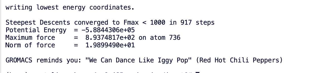
9. Sehen Sie sich die Ergebnisse an (am Ende des Tutorials zeigen wir Ihnen, wie Sie XVG-Dateien visualisieren. Sie können XMGrace, QTgrace, Python oder Excel verwenden, um ein Diagramm zu erstellen. Es handelt sich im Wesentlichen um ein Liniendiagramm.)
gmx_mpi energy -f em.edr -o potential.xvg
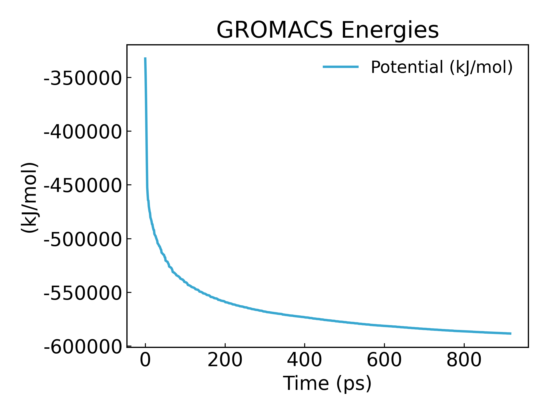
Man sieht, dass die Energie auf -600000 kj/mol minimiert wird
10. Systembalance
Ziel: Das System an die Zieltemperatur- und Druckbedingungen anpassen, um es dem realen physikalischen Zustand anzunähern.
(1) NVT-Simulation (konstantes Volumen und konstante Temperatur):
• Ein Ensemble aus konstantem Volumen und konstanter Temperatur wird verwendet, um die Temperatur des Systems auf einem Zielwert zu stabilisieren.
• Temperaturregler: Häufig werden Berendsen-Temperaturkoppler oder V-Rescale (modifizierte schwache Kopplungsmethode) verwendet, die die Temperatur durch Anpassung der Atomgeschwindigkeit regeln.
(2) NPT-Simulation (konstanter Druck und konstante Temperatur):
• Das Ensemble aus konstantem Druck und konstanter Temperatur passt die Systemdichte weiter an einen Zielwert an (normalerweise die Dichte von flüssigem Wasser ~1 g/cm³).
• Druckregler: Häufig werden Berendsen-Druckkoppler oder die Parrinello-Rahman-Druckregelmethode verwendet.
10.1. Führen Sie eine NVT-Äquilibrierung für 100 ps durch, die unter (konstanter Partikelanzahl, Volumen und Temperatur) durchgeführt wird, auch bekannt als "isotherm und isochor".
Mit GPU-Beschleunigung ist es sehr schnell und dauert nur mehr als 10 Sekunden.
gmx_mpi grompp -f nvt.mdp -c em.gro -r em.gro -p topol.top -o nvt.tpr

gmx_mpi mdrun -deffnm nvt -nb gpu -pme cpu
#将 PME 任务移至 CPU
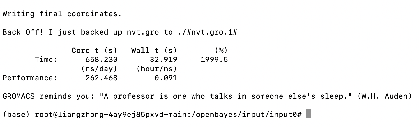
gmx_mpi energy -f nvt.edr -o temperature.xvg
#生成温度随时间变化的图像,查看温度是否平衡
16
0
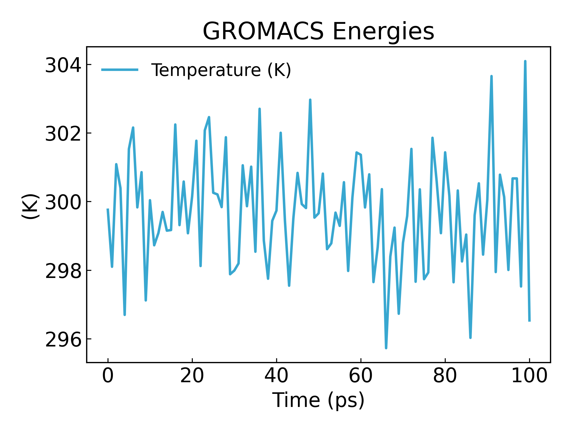
Es ist ersichtlich, dass die Temperatur innerhalb von 100ps ebenfalls einen stabilen Zustand erreicht.
10.2. NPT-„isothermer und isobarer“ Ausgleich, Stabilisierung des Systemdrucks und Durchführung eines 100-ps-NPT-Ausgleichs.
gmx_mpi grompp -f npt.mdp -c nvt.gro -r nvt.gro -t nvt.cpt -p topol.top -o npt.tpr
gmx_mpi mdrun -deffnm npt -nb gpu -pme cpu
#压力是否平衡
gmx_mpi energy -f npt.edr -o pressure.xvg
18
0
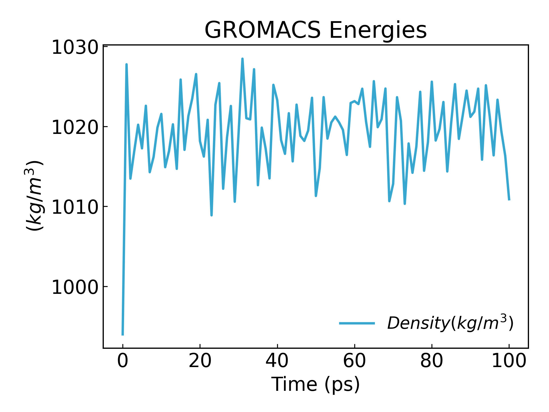
gmx_mpi energy -f npt.edr -o density.xvg
24
0
Wir können sehen, dass die Dichte einen stationären Zustand erreicht:
11. Nach Abschluss der beiden Gleichgewichtsphasen ist das System nun bei der gewünschten Temperatur und dem gewünschten Druck gut im Gleichgewicht. Wir können jetzt die Positionsbeschränkungen aufheben und MD ausführen, um fortzufahren.
Sie können die Zeit Ihren Bedürfnissen entsprechend ändern. Dieses Tutorial simuliert 100 ns.
Zeitschritt dt = 2 fs (übliche Einstellung):
50000000 Schritte, mit einem Zeitschritt von 2 fs, entsprechend 100 Nanosekunden (ns)
50000000 x 2 fs = 10^8 fs = 10^5 ps = 100 ns
vim md.mdp
nsteps                  = 50000000    ; 2 * 50000000 = 100000 ps (100 ns)
gmx_mpi grompp -f md.mdp -c npt.gro -t npt.cpt -p topol.top -o md_0_1.tpr

##最后一步提交,pme 分配到 CPU 上:
gmx_mpi mdrun -deffnm md_0_1 -v -nb gpu -pme cpu
-v kann die verbleibende Zeit des Laufs anzeigen.
3. Ergebnisanalyse
1. trjconv, das als Nachbearbeitungstool verwendet wird, um Koordinaten zu entfernen, die Periodizität zu korrigieren oder die Flugbahn manuell zu ändern (Zeiteinheit, Bildrate usw.). Dies liegt daran, dass bei allen Simulationen mit periodischen Randbedingungen Moleküle am Rand der Box abbrechen oder herumspringen können. Es kann das Molekül in der Box neu zentrieren, das Molekül neu einwickeln und die rhombisch-dodekaedrische Form der Box wiederherstellen.
-pbc mol: 去除轨迹中的周期性边界条件 (PBC),并基于分子进行修正(即确保每个分子在轨迹中是完整的)。
•	-center: 将选定的分子/分组居中到模拟框的中心。
gmx_mpi trjconv -s md_0_1.tpr -f md_0_1.xtc -o md_0_1_noPBC.xtc -pbc mol -center

Select group for centering
Group     0 (         System) has 33876 elements
Group     1 (        Protein) has  1960 elements
Group     2 (      Protein-H) has  1001 elements
Group     3 (        C-alpha) has   129 elements
Group     4 (       Backbone) has   387 elements
Group     5 (      MainChain) has   517 elements
Group     6 (   MainChain+Cb) has   634 elements
Group     7 (    MainChain+H) has   646 elements
Group     8 (      SideChain) has  1314 elements
Group     9 (    SideChain-H) has   484 elements
Group    10 (    Prot-Masses) has  1960 elements
Group    11 (    non-Protein) has 31916 elements
Group    12 (          Water) has 31908 elements
Group    13 (            SOL) has 31908 elements
Group    14 (      non-Water) has  1968 elements
Group    15 (            Ion) has     8 elements
Group    16 ( Water_and_ions) has 31916 elements
Select a group: 1
Selected 1: 'Protein'
Select group for output
Group     0 (         System) has 33876 elements
Group     1 (        Protein) has  1960 elements
Group     2 (      Protein-H) has  1001 elements
Group     3 (        C-alpha) has   129 elements
Group     4 (       Backbone) has   387 elements
Group     5 (      MainChain) has   517 elements
Group     6 (   MainChain+Cb) has   634 elements
Group     7 (    MainChain+H) has   646 elements
Group     8 (      SideChain) has  1314 elements
Group     9 (    SideChain-H) has   484 elements
Group    10 (    Prot-Masses) has  1960 elements
Group    11 (    non-Protein) has 31916 elements
Group    12 (          Water) has 31908 elements
Group    13 (            SOL) has 31908 elements
Group    14 (      non-Water) has  1968 elements
Group    15 (            Ion) has     8 elements
Group    16 ( Water_and_ions) has 31916 elements
Select a group: 0
Selected 0: 'System'
Auswahl 4 („Backbone“) wurde für die Kleinstquadrate-Anpassung und RMSD-Berechnungen verwendet.
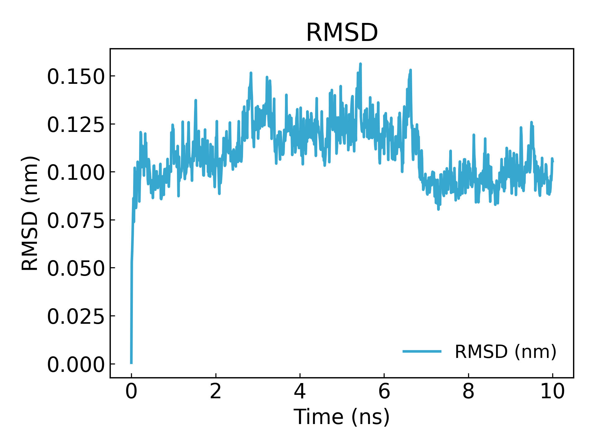
2. RMSD
Kann verwendet werden, um die Konvergenz der Simulation und die Stabilität des Proteins zu überprüfen.g_rms**Der RMSD der Struktur während der Simulation und der Anfangsstruktur, die Abweichung der Struktur zu einem bestimmten Zeitpunkt relativ zu 0 ns, wird häufig zur Bewertung der Stabilität der Proteinstruktur verwendet. Es wird häufig im Bereich der Arzneimittelentwicklung verwendet, beispielsweise zur Stabilität der Proteinligandenstruktur. Die Schwankungsbreite der RMSD-Kurve ist gering und stabil, was darauf hindeutet, dass die Affinität zwischen Ligand und Rezeptor groß ist.
gmx_mpi rms -s md_0_1.tpr -f md_0_1_noPBC.xtc -o rmsd.xvg
Wählen Sie 4 ("Backbone") für die Kleinstquadrate-Anpassung und RMSD-Berechnung
Es ist ersichtlich, dass das Gleichgewicht nach 10 ns erreicht ist (Hinweis: Beim Veröffentlichen oder Einreichen eines Artikels ist es am besten, 100 ns oder 50 ns zu simulieren).
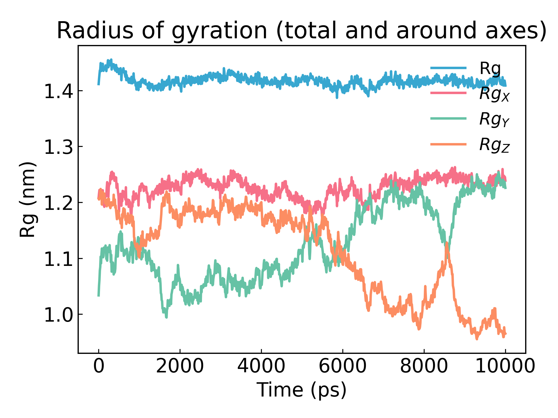
3. Trägheitsradiusanalyse
gmx_mpi gyrate -s md_0_1.tpr -f md_0_1_noPBC.xtc -o gyrate.xvg
Der Trägheitsradius eines Proteins ist ein Maß für seine Kompaktheit. Wenn eine Proteinstruktur stabil ist, behält sie wahrscheinlich einen relativ stabilen R g -Wert bei. Wenn sich ein Protein entfaltet, ändert sich sein R g -Wert mit der Zeit. Analysieren wir den Trägheitsradius von Lysozym in unserer Simulation:
4. Visualisierung
Empfohlene Software:DuIvyTools: GROMACS-Simulationsanalyse- und Visualisierungstools
Aus:https://github.com/CharlesHahn/DuIvyTools
pip install DuIvyTools

dit xvg_show -f rmsd.xvg -o rmsd_plot.png

dit xvg_show -f rmsd.xvg -o rmsd_plot.png

dit xvg_show -f potential.xvg -o potential_plot.png

dit xvg_show -f temperature.xvg -o temperature_plot.png

dit xvg_show -f density.xvg -o density_plot.png
dit xvg_show -f pressure.xvg -o pressure_plot.png
Öffnen Sie den von uns erstellten Datensatz
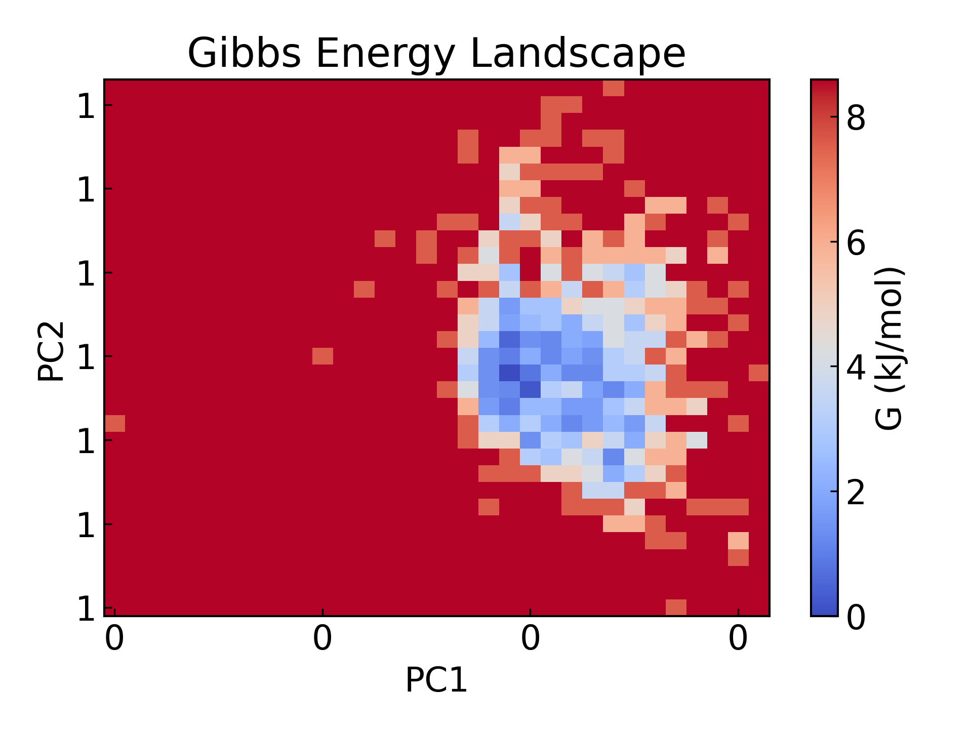
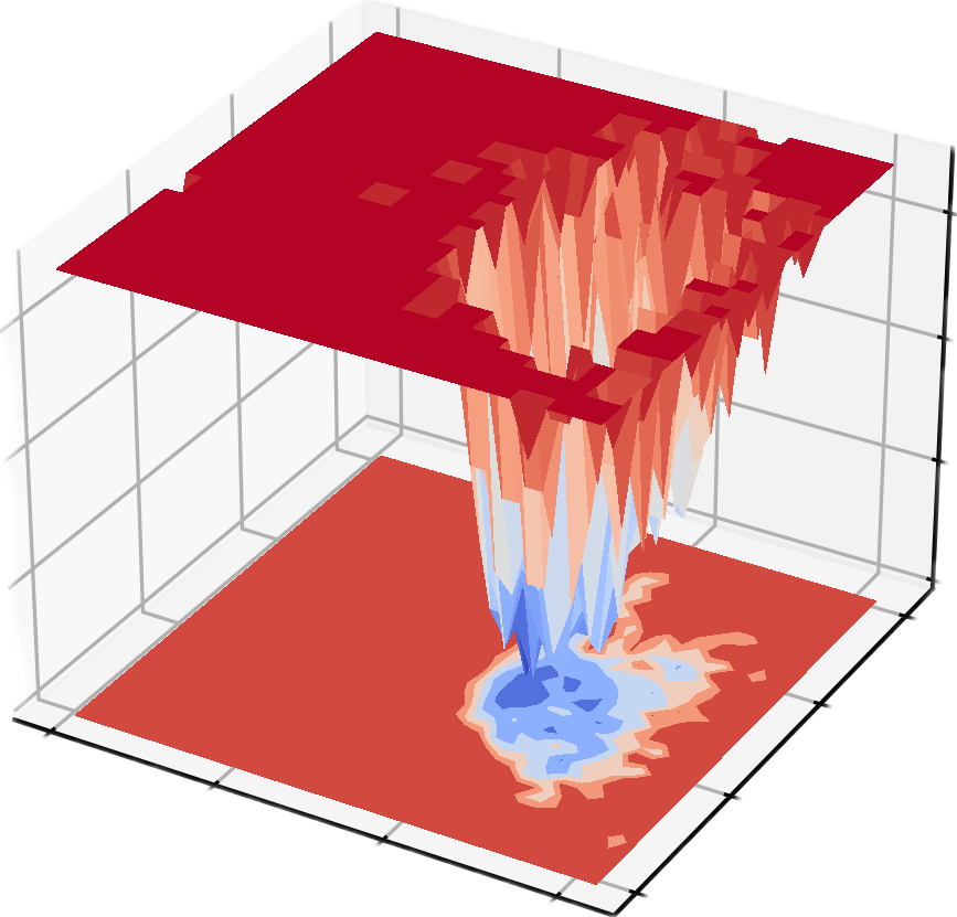
5. GROMACS-Energielandschaftskartierung Die freie Energielandschaft wurde mit dem Gyrationsradius und dem RMSD als zwei PCA-Komponenten dargestellt.
gmx_mpi gyrate -s md_0_1.tpr -f md_0_1_noPBC.xtc -o rg.xvg
gmx_mpi rms -s md_0_1.tpr -f md_0_1_noPBC.xtc -o rmsd.xvg
vim rmsd.xvg
#输入以下命令删除以 # 或 @ 开头的行:
:g/^[@#]/d

vim rg.xvg
#输入以下命令删除以 # 或 @ 开头的行:
:g/^[@#]/d

#注意不要有空行,
paste rmsd.xvg rg.xvg > rmsd-rg.xvg

(base) # tail -f rmsd-rg.xvg
9910.0000000    0.0925907	      9910     1.37624     1.20925     1.20765    0.931324
9920.0000000    0.0881348	      9920     1.38369     1.22248     1.21078    0.932077
9930.0000000    0.0911074	      9930     1.39224     1.23799     1.21709    0.928842
9940.0000000    0.0893596	      9940     1.38188     1.21942     1.21672    0.922916
9950.0000000    0.0915931	      9950     1.37509     1.21939     1.20194    0.922051
9960.0000000    0.0978161	      9960     1.38113      1.2262     1.21084    0.919414
9970.0000000    0.0954911	      9970     1.37934     1.21241     1.20711    0.937075
9980.0000000    0.0993617	      9980     1.38301     1.22353     1.21083     0.92862
9990.0000000    0.1069279	      9990     1.37943     1.22317     1.20579    0.924978
10000.0000000    0.1055321	     10000     1.37524     1.21648     1.20194     0.92632
^Z
[11]+  Stopped                 tail -f rmsd-rg.xvg
#查看已经将两个文件整合在一起了,我们只要保留
#从 rmsd-rg.xvg 文件内容可以看到,每一行的数据格式如下:
时间_RMSD(ns)    RMSD	      时间_Rg(ps)     Rg 其他列

(base) tail -f rmsd.xvg
9910.0000000    0.0925907
9920.0000000    0.0881348
9930.0000000    0.0911074
9940.0000000    0.0893596
9950.0000000    0.0915931
9960.0000000    0.0978161
9970.0000000    0.0954911
9980.0000000    0.0993617
9990.0000000    0.1069279
10000.0000000    0.1055321
^Z
[12]+  Stopped                 tail -f rmsd.xvg

#整理数据为
时间 (ns)    RMSD    Rg

(base) python
Python 3.8.15 (default, Nov 24 2022, 15:19:38)
[GCC 11.2.0] :: Anaconda, Inc. on linux
Type "help", "copyright", "credits" or "license" for more information.
# 加载数据
>>> import pandas as pd
>>> data = pd.read_csv("rmsd-rg.xvg", delim_whitespace=True, header=None, comment="#")
# 保留需要的列:第 1 列 (RMSD 时间) 、第 2 列 (RMSD) 、第 4 列 (Rg)
>>> cleaned_data = data[[0, 1, 3]]
# 将列名修改为更直观的名称
>>> cleaned_data.columns = ["Time (ps)", "RMSD", "Rg"]
>>> cleaned_data.to_csv("rmsd-rg-cleaned.xvg", sep="\t", index=False, header=False)
>>> exit()

#整理成功
tail -f rmsd-rg-cleaned.xvg
9910.0	0.0925907	1.37624
9920.0	0.0881348	1.38369
9930.0	0.0911074	1.39224
9940.0	0.0893596	1.38188
9950.0	0.0915931	1.37509
9960.0	0.0978161	1.38113
9970.0	0.0954911	1.37934
9980.0	0.0993617	1.38301
9990.0	0.1069279	1.37943
10000.0	0.1055321	1.37524

gmx_mpi sham -tsham 300 -nlevels 100 -f rmsd-rg-cleaned.xvg -ls gibbs.xpm -g gibbs.log -lsh enthalpy.xpm -lss entropy.xpm

dit xpm_show -f gibbs.xpm  -o gibbs_2d.png
dit xpm_show -f gibbs.xpm -m 3d -o gibbs_3d.png
#tsham : 设定温度
#-nlevels: 设定 FEL 的层次数量
Die Freie Energielandschaft (FES) ist ein sehr wichtiges Werkzeug in der Molekülsimulation, das hauptsächlich zur Beschreibung der freien Energieverteilung molekularer Systeme an bestimmten Koordinaten verwendet wird. Seine Hauptfunktion besteht darin, die thermodynamische Stabilität und den kinetischen Prozess des Systems aufzudecken, was in der Regel in den folgenden wissenschaftlichen Forschungsbereichen von großer Bedeutung ist:
- Steady-State- und Übergangszustandsstudien: Zeigen Sie die stabile Konformation (Punkt des freien Energieminimums) und den Konformationsumwandlungspfad (Barriere der freien Energie) des Systems auf, das zur Analyse der Proteinfaltung, chemischer Reaktionen und molekularer Erkennungsprozesse verwendet wird.
- Kinetische Wege und thermodynamische Stabilität: Die Quantifizierung der freien Energiedifferenz zwischen verschiedenen Zuständen hilft dabei, die energetische Antriebskraft molekularer Wechselwirkungen und Konformationsübergänge zu verstehen.
- Wirkstoffdesign und Katalyseforschung:Prognostizieren Sie Ligand-Rezeptor-Bindungswege, Energiebarrieren und Reaktionsraten und bieten Sie theoretische Anleitungen für die Analyse molekularer Mechanismen und die Funktionsoptimierung.
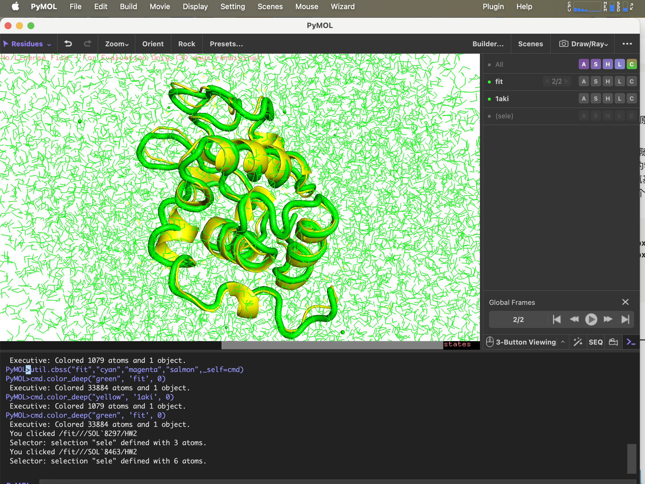
6.g_confrms Vergleich der Konformationsunterschiede
Um die Struktur nach der Simulation mit der Struktur in der ursprünglichen PDB-Datei zu vergleichen,fit.pdb Eine Datei mit zwei Molekülstrukturen, wählen Sie beide aus 4 (Backbone)
gmx_mpi confrms -f1 1AKI_clean.pdb -f2 md_0_1.gro -o fit.pdb
pdb-Struktur mit Pymol geöffnet
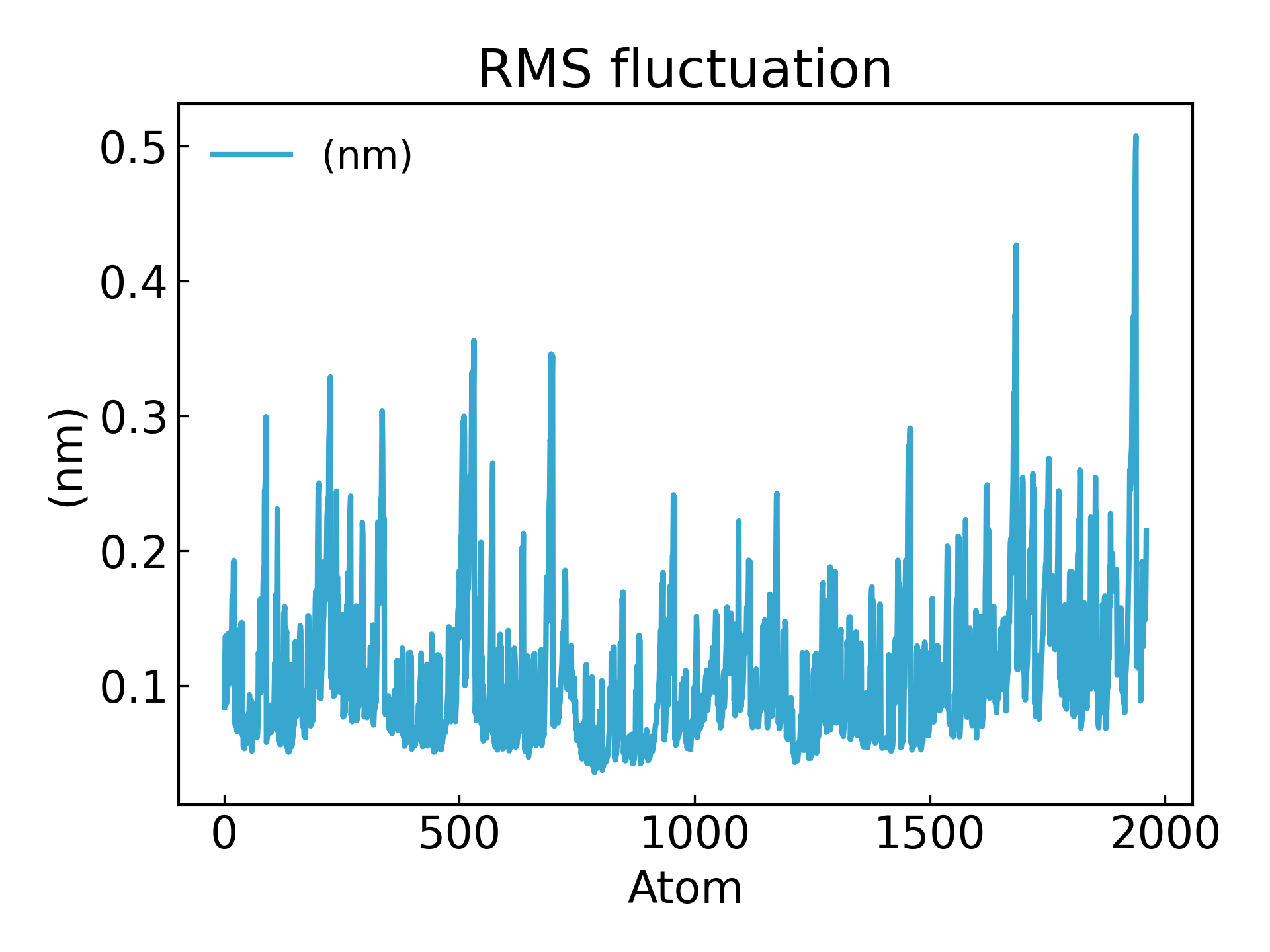
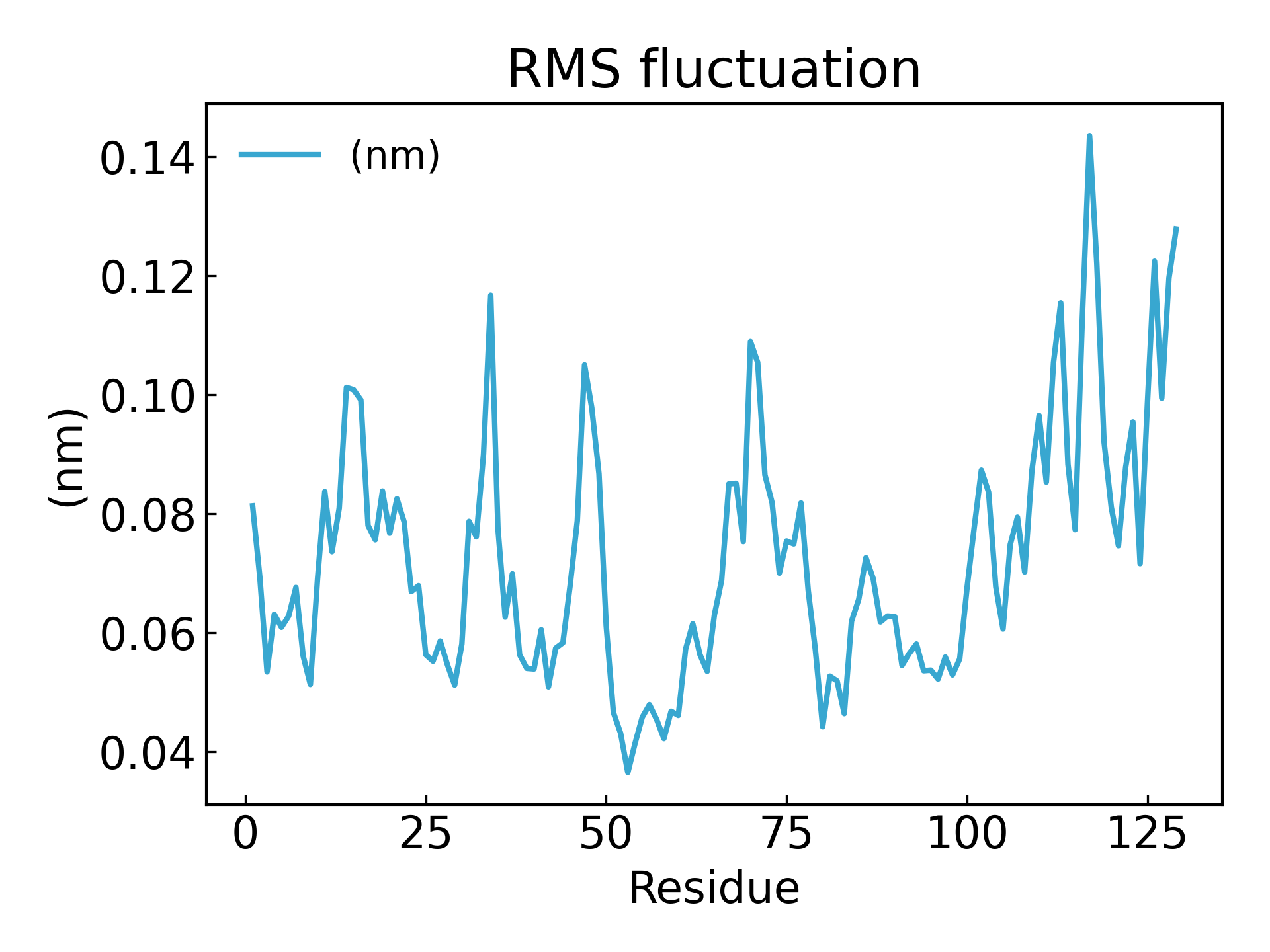
7.g_rmsf Berechnen Sie die quadratische Mittelwertfluktuation (RMSF) und die durchschnittliche Struktur innerhalb der nächsten 500 ps.g_rmsf Das Ergebnis ist eine Kurve, die sich mit der Ordnungszahl ändert. Wählen 1 Protein
Die Schwankungen der Aminosäurereste können mithilfe des RMSF-Parameters abgeleitet werden, der die durchschnittliche Abweichung jedes Aminosäurerests/-atoms von einer Referenzposition im Laufe der Zeit erklärt. Vielmehr handelt es sich dabei um die Analyse spezifischer Teile der Struktur eines Proteins, die von seiner durchschnittlichen Struktur abweichen. Aminosäuren oder Aminosäuregruppen mit hohen RMSF-Werten weisen darauf hin, dass der Komplex eine größere Flexibilität besitzt, während Aminosäuren mit niedrigeren RMSF-Werten darauf hinweisen, dass der Komplex eine geringere Flexibilität besitzt. Häufige Schwankungen führen zu einer schlechteren Stabilität. Der RMSF-Wert ist ein dynamischer Parameter, der zur Messung der durchschnittlichen Rückgratflexibilität jeder Restposition verwendet wird[19].
gmx_mpi rmsf -s md_0_1.tpr -f md_0_1_noPBC.xtc -b 500 -o fws-rmsf.xvg -ox fws-avg.pdb
gmx_mpi rmsf -s md_0_1.tpr -f md_0_1_noPBC.xtc -b 500 -o fws-rmsf.xvg -ox fws-avg.pdb -res

dit xvg_show -f fws-rmsf.xvg -o rmsf_res.png
# 最后可以放到 pymol 里面看轨迹动画,点击播放即可
gmx_mpi trjconv -s md_0_1.tpr -f md_0_1_noPBC.xtc -o trajectory.pdb -skip 10
Referenz
KI mit KI entwickeln
Von der Idee bis zum Launch – beschleunigen Sie Ihre KI-Entwicklung mit kostenlosem KI-Co-Coding, sofort einsatzbereiter Umgebung und bestem GPU-Preis.