Command Palette
Search for a command to run...
使用吉布斯扩散 (Gibbs-Diffusion) 进行图像盲降噪
基于 Gibbs-Diffusion 的图片盲去噪

教程简介
GDiff 全称 Gibbs-Diffusion,是一种贝叶斯盲去噪方法,解决了信号和噪声参数的后验采样问题。它依赖于吉布斯采样器,该采样器将采样步骤与预训练扩散模型(定义信号先验)和哈密顿蒙特卡罗采样器交替进行。论文介绍了其在自然图像去噪和宇宙学(宇宙微波背景分析)中的应用。论文成果为 Listening to the Noise: Blind Denoising with Gibbs Diffusion
官方文档中仅给出测试的方法,即传入清晰的原图,叠加噪声后再进行非盲去噪,盲去噪的对比。
效果演示
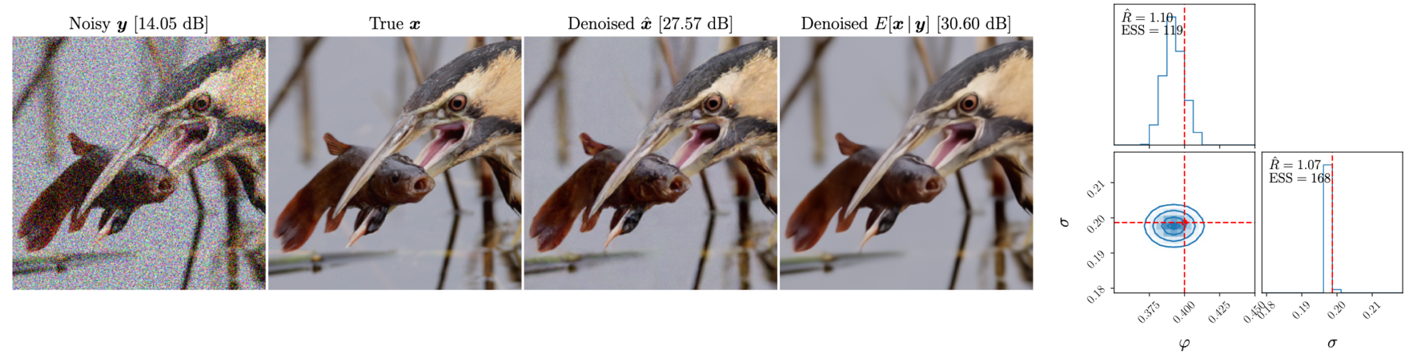
在官方的效果演示中,传入清晰的原图,对其叠加一定参数的噪声,然后再进行盲去噪。
下图从左到右依次为:叠加噪声后的图,原图,盲去噪效果图,去噪的后验均值
盲去噪与非盲去噪介绍
盲去噪(Blind Denoising)和非盲去噪(Non-Blind Denoising)是图像处理和信号处理中的两种去噪方法。它们主要的区别在于对噪声信息的预知程度。
盲去噪
定义:盲去噪是指在不知道噪声特性或噪声模型的情况下进行去噪处理。这种方法不依赖于对噪声的先验知识,而是通过图像或信号本身的信息来进行去噪。
特点:
- 不依赖噪声模型:无需知道噪声的类型、分布或强度。
- 自适应性强:可以应用于各种不同类型的噪声和信号环境。
- 复杂度高:由于没有噪声模型的帮助,盲去噪通常需要更复杂的算法和更多的计算资源。
非盲去噪
定义:非盲去噪是指在已知噪声特性或噪声模型的情况下进行去噪处理。这种方法利用对噪声的先验知识来优化去噪过程。
特点:
- 依赖噪声模型:需要预先了解噪声的类型、分布和强度等特性。
- 效果较好:在已知噪声模型的情况下,可以针对特定噪声类型进行优化,从而得到更好的去噪效果。
- 适用范围有限:对于不同类型的噪声,需要不同的模型和参数,适用范围较盲去噪狭窄。
教程运行方法
本教程分为两部分,第一部分为「模糊图片盲去噪」,在 start.ipynb 文件中可运行(即本文件),这里可以传入带有噪声的模糊图片,以进行盲去噪; 第二部分为「清晰图片叠加噪声与去噪清晰图片叠加噪声与去噪」,在 test.ipynb 文件中运行,这是官方文档的简化,可用于传入清晰图片叠加噪声,以此来对比盲去噪模型与非盲去噪的区别。
如需使用自定义图片,仅需上传图片并修改需要处理的图片的路径,依次运行即可。(图片名必须命名为英文)
第一部分:模糊图片盲去噪(start.ipynb)
导入需要的包
import sys, time
import torch
import numpy as np
import matplotlib.pyplot as plt
import corner
import arviz as az
from PIL import Image

sys.path.append('..')

from gdiff.data import ImageDataset, get_colored_noise_2d
from gdiff.model import load_model
import gdiff.hmc_utils as iut
from gdiff.utils import ssim, psnr, plot_power_spectrum, plot_list_of_images

plt.rcParams.update(
{
'text.usetex': False,
    'font.family': 'stixgeneral',
'mathtext.fontset': 'stix',
}
)
图片读取与预处理函数,使用方法来自官方文档 data.py
#图片读取与预处理,方法来自官方文档 data.py
def readimg(filename):
    from torchvision import transforms
    img=Image.open(filename)
    trans = transforms.Compose([transforms.Resize(256),
                                            transforms.CenterCrop(256),
                                            transforms.RandomHorizontalFlip(),
                                            transforms.ToTensor()])
    img=trans(img)
    return img
下面为官方读取数据集的方法,此文档中未使用。用户可在其文件夹中放入自己的数据集,稍作修改,即可实现批量处理(文件夹名只可以选给出的几种,在 data 文件夹中)
#
# PARAMETERS 官方数据读取与噪声参数,模型选择
#

# Dataset and sample 读取官方数据集
dataset_name = "CBSD68" # Choices among "imagenet_train", "imagenet_val", "CBSD68", "McMaster", "Kodak24"
dataset = ImageDataset(dataset_name, data_dir='./data')
sample_id = 0 # np.random.randint(len(dataset))

# Noise 准备叠在在清晰图片上的噪声
phi_true = -0.4     # Spectral index -> between -1 and 1 (\varphi in the paper)
sigma_true = 0.1    # Noise level

# Device
device = torch.device('cuda' if torch.cuda.is_available() else 'cpu')

# Model 选择模型,有 5000 与 10000 步迭代模型可选
diffusion_steps = 5000 # Number of diffusion steps: 5000 or 10000
model = load_model(diffusion_steps=diffusion_steps,
                   device=device,
                   root_dir='./model_checkpoints')
model.eval()

# Inference
num_chains = 4      # Number of HMC chains
n_it_gibbs = 50     # Number of Gibbs iterations after burn-in
n_it_burnin = 25    # Number of burn-in iterations
接下来,读入需要去噪处理的图片,例如,本教程使用的图片为 home 目录下的’3_noisy.png’,则在 img=readimg(‘3_noisy.png’) 处直接更改路径 ‘3_noisy.png’ 即可
在 A6000 单卡的情况下,单张图片的处理需要几分钟
#
# DENOISING 在此处读入的图片为高噪声图,在此处进行降噪处理
#

# 读取自己的高噪声图片,用于去噪
img=readimg('3_noisy.png')
x = img.to(device).unsqueeze(0)

# Our DDPM has discrete timestepping -> we get the time step closest to the chosen noise level
sigma_true_timestep, sigma_true = model.get_closest_timestep(torch.tensor([sigma_true]), ret_sigma=True)
alpha_bar_t = model.alpha_bar_t[sigma_true_timestep.cpu()].reshape(-1, 1, 1, 1).to(device)
print(f"Time step corresponding to noise level {sigma_true.item():.3f}: {sigma_true_timestep.item()}")
yt = torch.sqrt(alpha_bar_t) * x # Noisy image normalized for the diffusion model 归一化图像

# Non-blind denoising (for reference) 非盲去噪 即已知噪声参数的情况下去噪

print("Denoising in non-blind setting...")
t0 = time.time()
x_hat_nonblind = model.denoise_samples_batch_time(yt,
                                                  sigma_true_timestep.unsqueeze(0),
                                                  phi_ps=phi_true)
t1 = time.time()
print(f"Non-blind denoising took {t1-t0:.2f} seconds")

# Blind denoising with GDiff 基于 GDiff 的盲去噪
print("Denoising in blind setting (GDiff)...")
t0 = time.time()
phi_hat_blind, x_hat_blind = model.blind_denoising(x, yt,
                                                   num_chains_per_sample=num_chains,
                                                   n_it_gibbs=n_it_gibbs,
                                                   n_it_burnin=n_it_burnin)
t1 = time.time()
print(f"Blind denoising took {t1-t0:.2f} seconds")

# Denoised posterior mean estimate 去噪的后验均值估计
x_hat_blind_pmean = x_hat_blind[:, n_it_burnin:].mean(dim=(0, 1))
Time step corresponding to noise level 0.100: 134 Denoising in non-blind setting... Non-blind denoising took 4.48 seconds Denoising in blind setting (GDiff)...
0%| | 0/75 [00:00<?, ?it/s]
Adapting step size using 300 iterations
Step size fixed to :  tensor([0.0179, 0.0181, 0.0179, 0.0194], device='cuda:0')
100%|██████████| 75/75 [08:52<00:00, 7.10s/it]
Blind denoising took 532.30 seconds
#
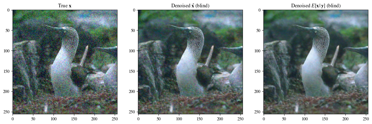
# Plot of a reconstruction 展示结果 顺序为:原始图片 非盲去噪 盲去噪 去噪的后验均值
#
data = [x[0],
x_hat_blind[0, -1],
x_hat_blind_pmean]
data = [d.to(device) for d in data]
labels_base = [r"True $\mathbf{x}$",
r"Denoised $\hat{\mathbf{x}}$ (blind)",
r"Denoised $E[\mathbf{x}\,|\,\mathbf{y}]$ (blind)"]
labels = [labels_base[0] ,
labels_base[1] ,
labels_base[2] ]
plot_list_of_images(data, labels)
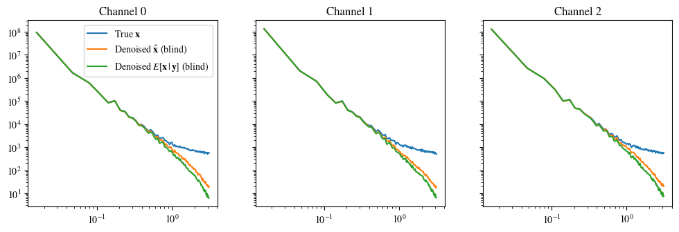
plot_power_spectrum(data, labels_base, figsize=(12, 3.5))Clipping input data to the valid range for imshow with RGB data ([0..1] for floats or [0..255] for integers).